How to backtest a strategy

A monthly momentum strategy backtested end to end in Python with the bt library, on simulated data, before and after trading costs.

A backtest estimates what a strategy would have earned in the past. Here I run a backtest from start to finish in Python with the bt library. I define a monthly momentum strategy, which buys the stocks with the highest past returns and uses only information available when it trades, and compare its result before and after a trading commission. On simulated data with momentum built in, it grows 9.1% a year before the commission and 8.6% after, against 4.6% for the market. The code needs pandas, matplotlib and bt.

Step 1. Loading the data

I test on simulated data, which needs no data subscription: almost six years of daily returns for 40 stocks. Each stock’s expected return has a part of its own that persists from day to day, so past returns predict future returns a little: the momentum the strategy looks for. I size it so that the tenth of stocks with the highest return over the past 12 months is expected to earn 1.33% a month more over the next three months than the tenth with the lowest, close to the 1.31% that Jegadeesh and Titman (1993) report for US stocks from 1965 to 1989. A separate script, make_returns.py, generated the returns and computes that expected difference. The block below loads its output, returns.csv, which has to be in the folder the code runs from. The box below gives the formula the script uses.

NoteHow the returns were simulated

Each stock’s daily return is a market move shared by all stocks, the stock’s own part of the expected return and noise,

\[r_{i,t} = m_t + e_{i,t} + \varepsilon_{i,t}, \qquad e_{i,t} = 0.997\,e_{i,t-1} + \sqrt{1 - 0.997^2}\;\sigma_e\,u_{i,t},\]

where the market move \(m_t\) is a draw from a bell-shaped normal distribution with a mean of 0.05% and a standard deviation of 1% a day, shared by all 40 stocks, and the noise \(\varepsilon_{i,t}\) is a normal draw with mean zero and a standard deviation of 1.2%, independent across stocks and days. The stock’s own part \(e_{i,t}\) starts as a normal draw with a standard deviation of \(\sigma_e = 0.05\%\) across stocks, and each day the own part keeps 99.7% of yesterday’s value and adds a standard normal draw \(u_{i,t}\), with a mean of 0 and a standard deviation of 1, independent across stocks and days, times \(\sqrt{1 - 0.997^2}\,\sigma_e\). A standard deviation measures how far values typically are from their mean. The two parts are independent, so their variances, the squared standard deviations, add up to \(0.997^2\sigma_e^2 + (1 - 0.997^2)\,\sigma_e^2 = \sigma_e^2\), and the spread of the own parts across stocks stays at 0.05% a day.

The own part’s expected value 231 trading days ahead is about half of today’s, since \(0.997^{231} \approx 0.5\). That persistence is the momentum, although the much larger daily noise makes past returns an imperfect guide. The market move, the noise and the persistence of 0.997 are assumptions.

The market move averages 0.05% a day, about 12.6% a year, and in this history the equal-weighted market of the 40 stocks grew at 4.6% a year, less by chance. The average of 1,512 daily moves with a standard deviation of 1% has a standard deviation of \(1\%/\sqrt{1{,}512} \approx 0.026\%\) a day, about 6.5% a year, and compounding lowers a growth rate below the average return.

NoteCode: the returns

import pandas as pd

# The dates are in the first column of the file. index_col=0 makes that column the row
# index, and parse_dates=True reads the text as real dates, so .date() works below.
returns = pd.read_csv("returns.csv", index_col=0, parse_dates=True)

number_of_days   = returns.shape[0]     # shape is (rows, columns), and one row is one day
number_of_stocks = returns.shape[1]     # one column is one stock
first_day = returns.index[0].date()     # .date() drops the midnight time stamp
last_day  = returns.index[-1].date()    # position -1 counts back from the end

print(f"{number_of_stocks} stocks x {number_of_days} trading days, "
      f"{first_day} to {last_day}")

# iloc selects by position, so this is the first five days and the first six stocks.
# print shows the table in a script as well as in a notebook.
corner_of_returns = returns.iloc[:5, :6].round(3)
print(corner_of_returns.to_string())

40 stocks x 1512 trading days, 2018-01-02 to 2023-10-18
            STK00  STK01  STK02  STK03  STK04  STK05
date                                                
2018-01-02  0.021 -0.008  0.013  0.013  0.008  0.000
2018-01-03 -0.012  0.001 -0.029  0.006 -0.021 -0.027
2018-01-04  0.013  0.006  0.016  0.005  0.007  0.028
2018-01-05  0.000  0.003 -0.013 -0.003  0.027 -0.029
2018-01-08 -0.034 -0.007 -0.021 -0.014 -0.003 -0.019

Each row is a day, each column a stock. Each value is that day’s return as a decimal: 0.01 is up one percent.

Step 2. Defining the strategy

Once a month I rank every stock by its return over the past year, keep the eight with the highest past-year return, divide the money equally among them and hold the shares until the next month. Price changes then move the weights away from equal until the next rebalance restores them.

A trade can only use data known before it. Ranking on the rebalance day’s close and trading at that same close would use a price not yet known when trading, which is look-ahead bias. So I lag the ranking by a day: rank on the latest close before the rebalance day, then trade at the rebalance day’s close. A longer lag also allows for data that arrives late.

In bt the strategy is a short list of steps, read top to bottom. The lag is one argument.

NoteCode: the strategies

import bt

# One year of calendar time does two jobs below: it is the history a stock needs before it
# can be ranked at all, and it is the period the momentum ranking is measured over.
RANKING_WINDOW = pd.DateOffset(months=12)
RANKING_LAG = pd.DateOffset(days=1)   # rank on the day before the trade, excluding the trade day

# bt runs this list in order on every day and stops as soon as a step returns False. That
# is how RunMonthly keeps the rest of the steps to one day a month.
momentum_steps = [
    bt.algos.RunMonthly(),                              # rebalance once a month
    bt.algos.SelectAll(),                               # consider every stock
    bt.algos.SelectHasData(lookback=RANKING_WINDOW,     # look back one year and require...
                           min_count=252),              # ...~252 valid daily prices before ranking
    bt.algos.SelectMomentum(n=8,                        # of those, keep the 8 with the highest...
                            lookback=RANKING_WINDOW,    # ...past-12-month return...
                            lag=RANKING_LAG),            # ...read up to the day BEFORE
    bt.algos.WeighEqually(),                            # weight those 8 equally
    bt.algos.Rebalance()]                               # trade to those weights

momentum = bt.Strategy("Momentum", momentum_steps)

# A benchmark to beat: hold all 40 stocks, equally weighted, rebalanced monthly. The same
# steps as above, without the two that pick and rank a subset.
market_steps = [
    bt.algos.RunMonthly(),
    bt.algos.SelectAll(),
    bt.algos.WeighEqually(),
    bt.algos.Rebalance()]

market = bt.Strategy("Market", market_steps)

SelectMomentum does not require a minimum number of observations, so SelectHasData before it requires 252 valid daily prices, about a trading year, so that every stock is ranked on about a year of history. In this complete panel every stock has that history by January 2019. In real data, the step would remove stocks that start trading later or have many missing days. The first trade comes a month later, in February 2019, because the strategy holds cash until its one-year ranking window lies entirely inside the data, and the headline statistics include that flat start.

Step 3. Running the backtest and charging for trading

bt works on prices, and the file holds returns, so the block first turns each stock’s daily returns into a price path starting at 100. Each day’s price is the previous day’s price times one plus that day’s return,

\[P_t = P_{t-1}\,(1 + r_t),\]

so, for example, a return of 1% and then one of −2% take 100 to 100 × 1.01 × 0.98 = 98.98. cumprod() repeats this multiplication down each stock’s column. The block then runs the momentum strategy twice, without a trading commission (gross) and with one (net), next to the benchmark.

Every month the strategy rebalances: it sells the stocks that left the top eight, buys the stocks that entered, and trades the rest back to equal weights. I charge a flat 10 basis points (0.10%) of each trade’s value, so the total cost grows with the value traded. In bt the charge is a small function passed as commissions.

NoteCode: the backtest

import io
import contextlib

# 1 + r is each day's growth factor, and cumprod multiplies the factors down each column
growth_factors = 1 + returns
prices = 100 * growth_factors.cumprod()     # each path is based at 100 dollars, so stocks are comparable


def trading_cost(quantity, price):
    """The commission bt charges on one trade: 10 basis points of its value.

    quantity is negative when the strategy sells, so abs treats a sale like a purchase.
    Selling 100 shares at 20 dollars costs 100 * 20 * 0.0010 = 2 dollars.
    """
    return abs(quantity) * price * 0.0010


# The same momentum strategy is run twice, once free of commission and once charged for
# it, so the difference between those two results is the cost of trading and nothing else.
momentum_gross = bt.Backtest(momentum, prices, name="Momentum",
                             integer_positions=False)
momentum_net = bt.Backtest(momentum, prices, name="Momentum_net",
                           commissions=trading_cost, integer_positions=False)
market_test = bt.Backtest(market, prices, name="Market",
                          integer_positions=False)

with contextlib.redirect_stderr(io.StringIO()):        # suppress bt's progress bar
    results = bt.run(momentum_gross, momentum_net, market_test)

integer_positions=False lets bt hold fractional shares, so the weights are exactly equal at each rebalance and no rounding to whole shares enters any of the three runs.

The Practical Coding section builds the same pieces in plain pandas: why the signal is lagged in lesson 30, and the whole backtest in one function in lesson 34.

Step 4. Reading the result

bt computes headline statistics for each run, in a table it calls stats. Momentum and Momentum_net are the same strategy, before and after the commission.

NoteCode: the headline statistics

# The stats table holds one row per measure and one column per run, so .loc picks the five
# rows worth showing here and keeps all three columns.
headline_measures = ["total_return", "cagr", "daily_sharpe", "max_drawdown", "calmar"]
headline_stats = results.stats.loc[headline_measures].round(3)
print(headline_stats.to_string())

              Momentum Momentum_net    Market
total_return  0.658037     0.616649  0.296259
cagr          0.091201      0.08645  0.045808
daily_sharpe  0.609221     0.582546  0.349611
max_drawdown  -0.18793     -0.18946  -0.22415
calmar        0.485294     0.456298  0.204365

total_return is the growth over the whole period: 65.8% for momentum before the commission, 61.7% after, and 29.6% for the market. cagr, the compound annual growth rate, is 9.1%, 8.6% and 4.6% a year. daily_sharpe is \(\sqrt{252}\,\bar r/s\), the average daily return \(\bar r\) divided by the standard deviation \(s\) of the daily returns, how far they typically are from their average, scaled to a year and without subtracting the risk-free rate, the return on cash (bt’s default): 0.61, 0.58 and 0.35. max_drawdown is the largest loss from a previous peak, 18.8%, 18.9% and 22.4%, and calmar is the CAGR divided by that loss, 0.49, 0.46 and 0.20.

The cost of trading depends on how much of the portfolio is traded, its turnover. bt measures a day’s turnover as the smaller of the purchases and the sales, divided by the portfolio’s value, while the commission is charged on both the purchases and the sales. Selling 20 and buying 20 in a portfolio worth 100 is a turnover of 20% and a commission of 0.001 × (20 + 20)/100 = 0.04% of the portfolio, twice the turnover times the commission rate. The next block reads the turnover from bt and measures the cost as the difference between the gross and the net CAGR.

NoteCode: the turnover and the cost

# bt's turnover is the smaller of the day's purchases or sales, divided by the portfolio's
# value. dropna guards against a day where that ratio cannot be formed, and this panel has none.
turnover = results.backtests["Momentum"].turnover.dropna()

# Turnover is zero between rebalances and on the first purchase, which sells nothing. A
# True/False mask inside .loc keeps the days with positive turnover, so the average is per
# rebalance after the first purchase rather than per calendar day.
rebalance_days = turnover > 0
average_turnover = turnover.loc[rebalance_days].mean()

gross = results.stats.loc["cagr", "Momentum"]       # yearly growth rate before costs
net = results.stats.loc["cagr", "Momentum_net"]     # the same run after the 10 bps charge
cost_in_cagr = (gross - net) * 100                  # the difference, in percentage points

print(f"Average turnover per rebalance: {average_turnover:.0%} of the portfolio")
print(f"Gross {gross:.1%}/yr  ->  net {net:.1%}/yr   "
      f"(cost in CAGR: {cost_in_cagr:.2f} percentage points/yr)")

Average turnover per rebalance: 22% of the portfolio
Gross 9.1%/yr  ->  net 8.6%/yr   (cost in CAGR: 0.48 percentage points/yr)

22% of the portfolio turns over at each monthly rebalance after the first purchase. At 10 basis points on both purchases and sales, each rebalance costs about \(2 \times 22\% \times 0.10\% \approx 0.04\%\) of the portfolio, and about twelve rebalances a year come to roughly half a percentage point: the difference in CAGR is 0.48 percentage points a year. The cost grows with turnover, so trading twice as much would roughly double the difference between gross and net. Real trading also pays the bid-ask spread, the gap between the price to buy and the price to sell, which a flat commission does not capture, so the true difference would be wider.

The chart below draws the value of each run over time.

NoteCode: the chart

import matplotlib.pyplot as plt

RED, TEAL, ORANGE, GREY = "#C0392B", "#17868A", "#D2822B", "#888888"
# The site's chart colours: a cream background, a light grid and a pale frame, so every chart
# on the site has the same look.
BG, INK, GRID, SPINE, AXIS_TEXT = "#FCEFE3", "#1f1f1f", "#EADCCC", "#D5C6B4", "#4a4a4a"


def style_chart(figure, axis):
    """Give a finished chart the site's cream background, light grid and pale frame."""
    figure.patch.set_facecolor(BG)
    axis.set_facecolor(BG)
    axis.grid(True, axis="y", color=GRID, lw=1.0)
    axis.set_axisbelow(True)
    for side in ("top", "right"):
        axis.spines[side].set_visible(False)
    for side in ("left", "bottom"):
        axis.spines[side].set_color(SPINE)
    axis.tick_params(axis="both", length=0, colors=INK, pad=6)
    axis.xaxis.label.set_color(AXIS_TEXT)
    axis.yaxis.label.set_color(AXIS_TEXT)
    axis.title.set_color(INK)
    # Each legend entry in the colour of what it labels: a line's colour or a bar's fill.
    # get_legend() returns None when the chart has no legend.
    legend = axis.get_legend()
    if legend is not None:
        for text, handle in zip(legend.get_texts(), legend.legend_handles):
            if hasattr(handle, "get_color"):
                text.set_color(handle.get_color())
            else:
                text.set_color(handle.get_facecolor())


# bt draws all three equity curves at once and passes the colours on to pandas, one per run
axis = results.plot(title="Momentum vs market (simulated data)", color=[TEAL, ORANGE, GREY])
axis.set_ylabel("value, starting at 100")
axis.legend(frameon=False)
style_chart(axis.get_figure(), axis)

# Saved to disk because the file is also the thumbnail the post lists in its frontmatter
plt.savefig("momentum_backtest_simulated.png", dpi=120, bbox_inches="tight", facecolor=BG)
plt.show()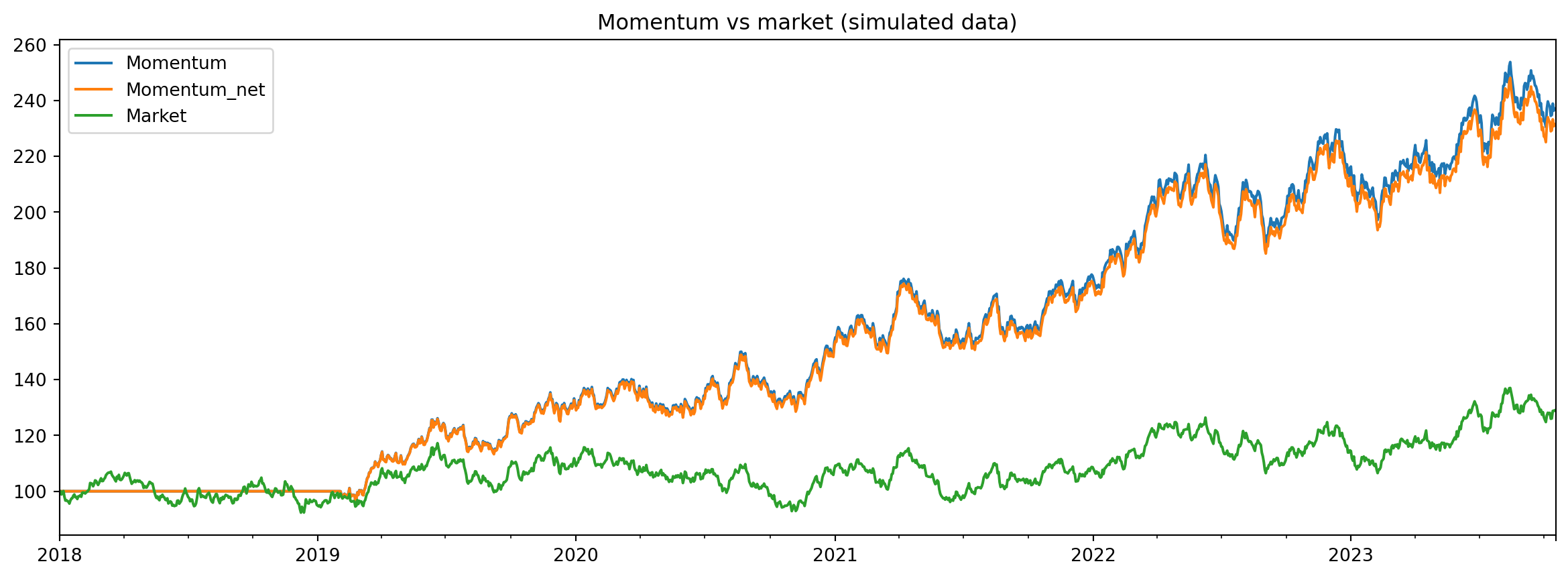

The teal and orange lines are the momentum strategy before and after the commission, and the grey line is the market. Momentum beat the market before and after the commission. The momentum built into the simulation makes that likely, and one simulated history cannot guarantee it. The gap between the teal and orange lines is the cost of trading, the one friction in this backtest. Each issue below either lowers the expected result or makes it less certain.

Limitations

Slippage. Slippage is the difference between the price a backtest assumes and the price a trade gets. Fills are usually worse than the quoted price, more so in less liquid stocks, which trade in smaller amounts. The 10 basis points I charged are an assumption, and often too low for illiquid stocks.

Capacity. Larger trades move the price against us, which is called price impact. The backtest assumes that our trades move no prices.

Overfitting. I tested one idea. A strategy chosen after testing many can fit the noise in historical data and then underperform once it trades.

Real data is messier. This panel is clean by construction. Real data has missing days, delistings, and erroneous prices. Cleaning it is a separate task.

One path, one planted edge. This is one simulated history, with momentum built in on purpose. Many simulated histories would give a distribution of outcomes, and none of them shows whether momentum works in a real market.

The takeaway is that a backtest is an estimate: lagging the ranking and charging for trades make it more realistic, and the issues above still make it uncertain.

Disclaimer: a teaching example on synthetic data. The returns here were generated, and the edge was planted on purpose. Not investment advice. Past performance does not guarantee future returns.

Sources: Narasimhan Jegadeesh and Sheridan Titman, Returns to Buying Winners and Selling Losers: Implications for Stock Market Efficiency, Journal of Finance 48(1), 65-91 (1993), Table I.