A set of short Python lines to backtest a strategy.
Published
June 8, 2026
Backtests are useful, but, as with all estimates, they contain uncertainty. More realistic assumptions reduce the risk of overstating what a strategy could have earned in practice. A backtest is still a historical estimate, not a forecast. But it helps us organize information and test whether an idea is plausible.
Here I run one end to end with the bt library. Four steps: load the data, define the strategy, run it, read the result. I also consider the cost of trading, so the headline number is more honest given the data.
Step 1. Load the data
We test on simulated data. Six years of daily returns for 40 stocks, with a momentum edge built in, so there is something for the strategy to find. Simulating it keeps the post reproducible and needs no data subscription. It is saved as a CSV. We load it.
import pandas as pdreturns = pd.read_csv("returns.csv", index_col=0, parse_dates=True) # the dates become the row indexprint(f"{returns.shape[1]} stocks x {returns.shape[0]} trading days, "f"{returns.index[0].date()} to {returns.index[-1].date()}")returns.iloc[:5, :6].round(3) # a corner of the table
40 stocks x 1512 trading days, 2018-01-02 to 2023-10-18
STK00
STK01
STK02
STK03
STK04
STK05
date
2018-01-02
0.022
-0.009
0.013
0.013
0.008
0.001
2018-01-03
-0.011
0.001
-0.030
0.006
-0.021
-0.026
2018-01-04
0.013
0.006
0.016
0.005
0.007
0.029
2018-01-05
0.001
0.003
-0.013
-0.003
0.027
-0.029
2018-01-08
-0.034
-0.007
-0.022
-0.014
-0.003
-0.019
Each row is a day, each column a stock. Each value is that day’s return as a decimal: 0.01 is up one percent.
Step 2. Define the strategy
The idea I want to test is momentum: past winners keep winning. Once a month we rank every stock by its return over the past year, keep the eight strongest, and hold them equally weighted until the next month.
Importantly, your decision can only use data from before the moment you trade. If the ranking uses the rebalance day itself, that is look-ahead bias, and the result is not optimistic, it is wrong. So we lag by a day. Rank using the latest available close before the rebalance, then trade at today’s close. If anything, we may need more lag, not less, since data retrieval can be delayed. A data vendor refreshes overnight. Thus, lagging is the safe default.
In bt the strategy is a short list of steps, read top to bottom. The lag is one argument.
import btmomentum = bt.Strategy("Momentum", [ bt.algos.RunMonthly(), # rebalance once a month bt.algos.SelectAll(), # consider every stock bt.algos.SelectHasData(lookback=pd.DateOffset(months=12), # look back one year and require... min_count=252), # ...~252 valid daily prices before ranking bt.algos.SelectMomentum(n=8, # of those, keep the 8 with the highest... lookback=pd.DateOffset(months=12), # ...past-12-month return... lag=pd.DateOffset(days=1)), # ...read up to the day BEFORE (no look-ahead) bt.algos.WeighEqually(), # weight those 8 equally bt.algos.Rebalance()]) # trade to those weights# A benchmark to beat: hold all 40 stocks, equally weighted, rebalanced monthly.market = bt.Strategy("Market", [bt.algos.RunMonthly(), bt.algos.SelectAll(), bt.algos.WeighEqually(), bt.algos.Rebalance()])
SelectHasData is a safety net that requires about a trading year of valid prices before a stock can be ranked. So the strategy holds cash until it has that history. The first trade here is February 2019, and the headline numbers cover the whole period, including that flat start. SelectMomentum ranks, but it does not enforce a minimum number of observations. SelectHasData does, thus forcing every stock to be ranked on roughly the same amount of history.
Step 3. Run it, and charge for trading
bt works on prices, not returns. So first I compound the returns into a price path. I scale each compounded price path by 100. Then I run momentum two ways, gross and after costs, next to the benchmark.
Now the cost. Every month, the strategy rebalances. It sells the names that left the top eight and buys the ones that entered it. That is turnover, and every trade pays. I charge a flat 10 basis points of each trade’s value. When turnover is low, the cost is small. When turnover is high, it is large. The cost scales with turnover. In bt it is a one-line commissions function.
import io, contextlibprices =100* (1+ returns).cumprod() # returns -> a $100 price path per stockcost =lambda quantity, price: abs(quantity) * price *0.0010# 10 bps of each trade's valuetests = [bt.Backtest(momentum, prices, name="Momentum", integer_positions=False), # gross bt.Backtest(momentum, prices, name="Momentum_net", commissions=cost, integer_positions=False), # after costs bt.Backtest(market, prices, name="Market", integer_positions=False)] # benchmarkwith contextlib.redirect_stderr(io.StringIO()): # hide bt's progress bar res = bt.run(*tests)
Note: integer_positions=False holds fractional shares, so the equal weights are exact. Rounding to whole shares then does not distort the costed run.
Step 4. Read the result
bt computes the headline stats for each run. Momentum and Momentum_net are the same strategy, before and after costs.
How much did the trading cost? That depends on how much we traded. So ask bt for the turnover, and read the cost off the gross-versus-net gap.
turnover = res.backtests["Momentum"].turnover.dropna() # bt's daily turnover; nonzero on rebalance daysgross = res.stats.loc["cagr", "Momentum"]net = res.stats.loc["cagr", "Momentum_net"]print(f"Average turnover per rebalance: {turnover[turnover >0].mean():.0%} of the book")print(f"Gross {gross:.1%}/yr -> net {net:.1%}/yr (CAGR drag: {(gross - net) *100:.2f} percentage points/yr)")
Average turnover per rebalance: 21% of the book
Gross 16.0%/yr  ->  net 15.6%/yr   (CAGR drag: 0.48 percentage points/yr)
About a fifth of the book turns over each month. At 10 bps that is half a percent a year. Small here. But it scales with turnover. Trade twice as often, or hold names with wider spreads, and the gap between gross and net widens quickly.
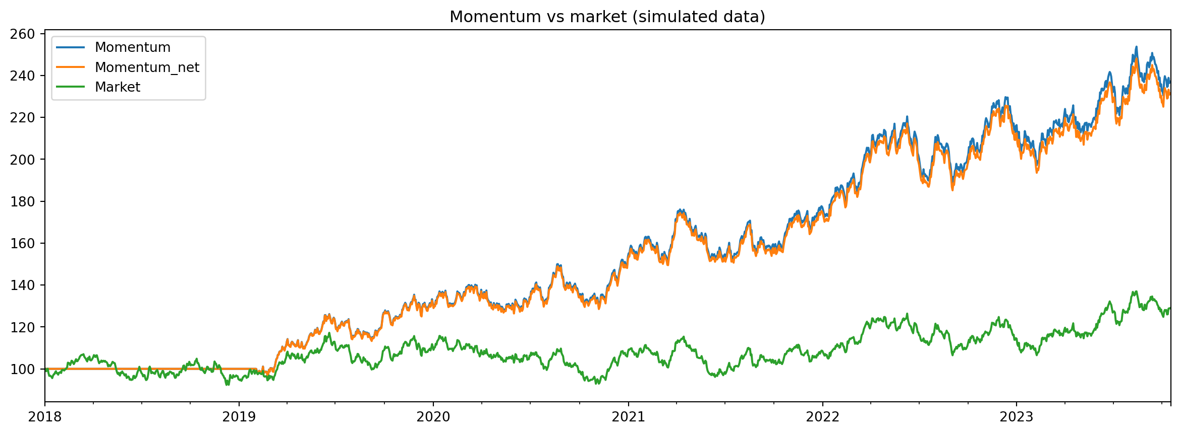
import matplotlib.pyplot as pltres.plot(title="Momentum vs market (simulated data)") # the equity curves, in one callplt.savefig("momentum_backtest_simulated.png", dpi=120, bbox_inches="tight")plt.show()
The backtest supports the prior. Momentum beat the market, before costs and after. The gap between the two momentum lines is the cost of trading, the one friction I put in. Note that the net line is a historical estimate under the discussed assumptions, not a future guarantee of performance. The following lowers the expected result or makes it less certain.
Issues to be aware of when backtesting
Slippage. Fills are usually worse than the quoted price, and the gap is wider in less liquid stocks. The 10 bps I charged is illustrative, and often too low for illiquid names.
Capacity. More capital invested increases the risk of price impact. The backtest does not incorporate your own price impact.
Overfitting. I tested one idea. The risk is that a strategy looks perfect on historical data, then underperforms once you implement it. The signal a backtest finds may just be noise.
Real data is messier. This panel is clean by construction. Real data has missing days, delistings, and erroneous prints. Cleaning it is a separate task.
One path, one planted edge. This is one simulated history, and the edge was added by construction. A single path gives one outcome. Many draws would give a distribution. Whether momentum works in a real market is something the simulation cannot answer.
A backtest narrows down what is plausible. That is useful. It does not promise the top of the range.
Disclaimer: a teaching example on synthetic data. The returns here were generated, not observed, and the edge was planted on purpose. Not investment advice. Past performance does not predict future returns.