import numpy as np                      # arrays + random number generation
import pandas as pd                     # tabular containers for clean reporting
from scipy.optimize import minimize     # numerical optimizer for maximum likelihood
import matplotlib.pyplot as plt         # plots

np.random.seed(42) # fixed seed for reproducibilityEstimating the Frequency of Market Crimes
Python
Code
Using Detection-Controlled Estimation to recover hidden market crimes from observed prosecutions.

To know whether a model works, we usually need the truth.
If I predict tomorrow’s return, I can compare the prediction with the actual return. If I classify trades as buys or sells, I can compare against the true trade direction. If I estimate execution costs, I need a benchmark for the true cost.
Market crime is harder. We observe prosecutions, but we do not observe all crimes. So we do not know how many crimes were missed, and we do not know how accurate the surveillance system really is.
A low number of prosecutions can mean two very different things. It can mean there were few crimes. Or it can mean many crimes happened and few were detected.
That is the problem Detection-Controlled Estimation (DCE) tries to solve. Patel and Putniņš (2020) use it to estimate how much insider trading happens around M&A and earnings announcements; Comerton-Forde and Putniņš (2014) use it to estimate the prevalence of closing-price manipulation. Both papers show that there are many more market crimes than there are prosecutions.
In this post, I show how to code DCE in Python to estimate the frequency of market crimes (here, illegal insider trading). I start by constructing a synthetic dataset where I know the truth: I decide how many crimes happen, how many are detected, and which cases become prosecutions. Then I hide the true crime and detection variables from the estimator and give DCE only what we would observe in real data (prosecutions and covariates).
Why prosecutions are not enough
Every announcement has two hidden steps. First, \(P(\text{crime})\), did insider trading happen? Second, \(P(\text{detection} \mid \text{crime})\), if it happened, was it detected and prosecuted?
What we observe is only the joint outcome:
\[P(\text{prosecution}) = P(\text{crime}) \times P(\text{detection} \mid \text{crime})\]
A 5% prosecution rate can come from many worlds:
| Crime rate | Detection rate | Prosecution rate |
|---|---|---|
| 5% | 100% | 5% |
| 10% | 50% | 5% |
| 25% | 20% | 5% |
| 50% | 10% | 5% |
The observed data are identical in all four. Prosecutions tell us the product; they do not tell us the two components. So we cannot stare at prosecution counts and answer “how much market crime is there?”
We also never observe true negatives or false negatives, both hide inside the non-prosecuted group, so accuracy can’t be computed the usual way. All we see, per the announcement, is whether a prosecution followed.
DCE tries to split that product.
What DCE adds
DCE adds structure. It estimates two equations at the same time. One explains the probability that a crime happened. The other explains the probability that the crime was detected, conditional on it happening.
The model needs variables that help separate the two. Some should mainly move the crime probability, in insider trading, the value of the information or how many people had access to it. Others should mainly move detection—surveillance signals, abnormal trading patterns, or regulatory resources. Some affect both: liquidity is the obvious example, since it can make trading easier to hide but can also change how suspicious a trade looks. Those both-side variables can be included as controls, but they do not do the clean identifying work.
The difficulty is whether the variables separate crime from detection, and if a variable you called “crime-only” actually also moves detection, the prosecution rate will still fit fine, while the split between the two gets quietly biased. More on that at the end.
The setup
I start by constructing a known world. Features are generated through a latent-factor structure, so they carry realistic correlations (bigger firms have bigger deals and more liquidity), not independent noise. Crime and detection outcomes are drawn from coefficients I choose. Then I hide everything except the features and the prosecution indicator, hand that to DCE, and check how close it lands to the truth I built.
This is the standard Monte Carlo framework (Hansen 2022, ch. 9.18). The exclusion restrictions are true by construction, which makes this a fair test of the mechanics, not a test of whether real-world exclusion arguments are credible.
Step 1. Build a known world
Five observable features. Two crime-side, two detection-side, one that loads on both. Then two latent logistic equations generate the true probability of crime and the true conditional probability of detection, and Bernoulli draws turn those into realized outcomes.
N = 10000  # number of announcements

# --- Latent factors that induce realistic correlations across features ---
firm_size_factor     = np.random.normal(0, 1, N)  # bigger firms: bigger deals + more liquidity
detection_era_factor = np.random.normal(0, 1, N)  # periods of stronger enforcement

# --- Five observable features ---
# Crime-side: correlated with firm size
info_value          = 0.7 * firm_size_factor     + 0.7 * np.random.normal(0, 1, N)
leakage             = 0.6 * firm_size_factor     + 0.8 * np.random.normal(0, 1, N)
# Detection-side: correlated with enforcement era
surveillance_signal = 0.7 * detection_era_factor + 0.7 * np.random.normal(0, 1, N)
reg_resources       = 0.8 * detection_era_factor + 0.6 * np.random.normal(0, 1, N)
# Both-side: also loads on firm size
liquidity           = 0.5 * firm_size_factor     + 0.9 * np.random.normal(0, 1, N)

# Standardize so coefficients have comparable magnitudes
def std_(x): return (x - x.mean()) / x.std()
info_value, leakage = std_(info_value), std_(leakage)
surveillance_signal, reg_resources = std_(surveillance_signal), std_(reg_resources)
liquidity = std_(liquidity)

# --- True coefficients (the truth we hide from DCE) ---
ic, b_info, b_leak, b_liq_c = -1.5, 0.9, 0.6, 0.4    # crime equation
id_, b_surv, b_reg, b_liq_d = -1.8, 1.2, 0.7, -0.3   # detection equation

def sigmoid(x): return 1.0 / (1.0 + np.exp(-x))
p_true = sigmoid(ic  + b_info*info_value          + b_leak*leakage      + b_liq_c*liquidity)
d_true = sigmoid(id_ + b_surv*surveillance_signal + b_reg*reg_resources + b_liq_d*liquidity)

# Realize crime and (conditional) detection via Bernoulli draws
C          = (np.random.uniform(0, 1, N) < p_true).astype(int)  # 1 = crime happened
D_if_crime = (np.random.uniform(0, 1, N) < d_true).astype(int)  # 1 = would be caught IF a crime happened
A          = C * D_if_crime                                      # 1 = prosecution (ONLY A is observable)

print("TRUTH (hidden from DCE):")
print(f"  mean P(crime)             = {p_true.mean():.2%}")
print(f"  mean P(detection | crime) = {d_true.mean():.2%}")
print()
print("OBSERVED (the only thing DCE sees, alongside the features):")
print(f"  P(prosecution)            = {A.mean():.2%}")
print(f"  P(no prosecution)         = {1 - A.mean():.2%}")
TRUTH (hidden from DCE):
mean P(crime) = 25.30%
mean P(detection | crime) = 22.93%
OBSERVED (the only thing DCE sees, alongside the features):
P(prosecution) = 4.97%
P(no prosecution) = 95.03%Two things to notice. The true crime rate is about 25% but the prosecution rate is only about 5%, so most crime in this world is never caught. And A = C * D_if_crime is the only column DCE gets to see. The crime label C and the detection label D_if_crime are hidden.
Step 2. The likelihood
The unit of observation is an announcement, a single dated, price-sensitive event, like a merger bid or an earnings release. It is a moment where someone could trade on inside information, it can be tied to a specific prosecution if one follows, and we can attach features to it.
Each announcement carries two hidden probabilities:
- \(p\) — the probability a crime happened, written as a logistic function of the crime-side features, \(p = \sigma(X_1 \beta_1)\).
- \(d\) — the probability the crime was detected given that it happened, \(d = \sigma(X_2 \beta_2)\).
The sigmoid \(\sigma\) just maps a weighted sum of features into a probability between 0 and 1. Two feature sets, two coefficient vectors, two probabilities per announcement.
Now the part we actually observe. Every announcement falls into exactly one of two groups: it was prosecuted (\(A = 1\)) or it was not (\(A = 0\)). The two groups are mutually exclusive and cover everything, so their probabilities sum to one. That partition gives us a probability we can write down.
A prosecution needs both a crime and its detection, so its probability is the product:
\[P(A = 1) = p \cdot d.\]
Everything else falls in the not-prosecuted group, either no crime, or a crime that went undetected, which carries the leftover probability:
\[P(A = 0) = 1 - p \cdot d.\]
So each announcement contributes \(p \cdot d\) if it was prosecuted and \(1 - p \cdot d\) if it was not. Multiply those contributions across all announcements and take logs, and the full-sample log-likelihood is
\[\log L = \sum_{i:\,A_i = 1} \log(p_i d_i) \;+\; \sum_{i:\,A_i = 0} \log(1 - p_i d_i).\]
Before the code, the question that matters is why each feature goes where it goes. The model is answering two different questions, what makes a crime more likely, and, given that a crime happened, what makes it more likely to be detected, so each feature has to be assigned to the question it actually bears on.
The five synthetic features split like this:
info_value— crime side. The more valuable the information, the larger the payoff from trading on it, and the more tempting the crime.leakage— crime side. The more people who hold the information, the more potential sources of illegal trading.surveillance_signal— detection side. It stands for the kind of abnormal pre-announcement trading that makes a case easier to notice. It does not prove a crime; the claim is only that given a crime, abnormal trading makes detection more likely.reg_resources— detection side. More enforcement resources make detection and prosecution easier.liquidity— both. This is the messy one. Liquidity makes illegal trading easier to hide, which is a crime-side effect, but it also shapes what looks abnormal to a surveillance system, which is a detection-side effect. Because it plausibly moves both, it cannot help separate them, it goes in as a control, not as an identifying variable.
These assignments are the economic assumptions of the model. What matters most is what each equation leaves out. The crime equation excludes surveillance_signal and reg_resources; the detection equation excludes info_value and leakage. Those exclusions are the exclusion restrictions, and they are what let the model pull the prosecution probability apart into a crime piece and a detection piece.
X1 = np.column_stack([np.ones(N), info_value,          leakage,       liquidity])
X2 = np.column_stack([np.ones(N), surveillance_signal, reg_resources, liquidity])
k1, k2 = X1.shape[1], X2.shape[1]

def dce_nll(params):
    b1, b2 = params[:k1], params[k1:]
    p = sigmoid(X1 @ b1)
    d = sigmoid(X2 @ b2)
    pd_prod = np.clip(p * d, 1e-12, 1 - 1e-12)          # guard the logs
    return -np.sum(A * np.log(pd_prod) + (1 - A) * np.log(1 - pd_prod))
Why fit both equations at once? Because we never observe either one on its own. There is no column that says “a crime happened,” and none that says “a crime happened but was missed.” We only observe whether each announcement was prosecuted (\(A = 1\)) or not (\(A = 0\)), and that single bit is the product of the two probabilities. A prosecution has to pass through both branches, a crime that occurred and was detected, so \(P(A_i = 1) = p_i d_i\). A not-prosecuted announcement is ambiguous: it could mean no crime, or a crime that escaped detection.
That ambiguity is what maximum likelihood has to resolve: it searches for the two sets of coefficients that make the observed prosecuted / not-prosecuted split most likely. But many \((p, d)\) pairs multiply to the same prosecution rate, a high-crime, low-detection world looks identical to a low-crime, high-detection world in prosecution data alone. The exclusion restrictions break that tie. They tell the optimizer which variation should move crime, which should move detection, and which is allowed to move both. Without them, DCE is barely more than a model of the prosecution rate; with them, it can estimate the hidden crime and detection pieces separately.
Results
The hidden crime probability is about 25%. But the observed prosecution rate is only about 5%. So if I only counted prosecutions, I would say market crimes happen in roughly 5% of announcements. That would be wrong, because most crimes in this synthetic world are never detected. DCE gives a different number. It estimates the crime rate at about 23% and the detection rate at about 24%. That is close to the hidden probabilities I used to generate the data.
That does not prove DCE works in real markets. It only shows that the likelihood works in a world where the assumptions are true. One run can still be lucky. So the next step is to repeat the whole experiment many times.
Does it work on average? Monte Carlo
The proper test re-runs the whole experiment many times and reports bias (does DCE systematically over- or under-estimate?) and RMSE (how far is a typical estimate from the truth?), following Hansen (2022, ch. 9.18) and Morris, White & Crowther (2019). Below: 200 independent replications, fresh synthetic data each time, N = 5,000 to keep runtime under a minute.
R_REPS = 200    # number of Monte Carlo replications
N_MC   = 5000   # sample size per replication

def run_one(seed):
    """Generate a fresh synthetic sample, fit DCE, return key aggregates."""
    rng = np.random.default_rng(seed)
    fs = rng.normal(0, 1, N_MC)
    de = rng.normal(0, 1, N_MC)
    iv = std_(0.7*fs + 0.7*rng.normal(0, 1, N_MC))
    lk = std_(0.6*fs + 0.8*rng.normal(0, 1, N_MC))
    ss = std_(0.7*de + 0.7*rng.normal(0, 1, N_MC))
    rr = std_(0.8*de + 0.6*rng.normal(0, 1, N_MC))
    lq = std_(0.5*fs + 0.9*rng.normal(0, 1, N_MC))
    p_t = sigmoid(ic  + b_info*iv + b_leak*lk + b_liq_c*lq)
    d_t = sigmoid(id_ + b_surv*ss + b_reg*rr  + b_liq_d*lq)
    C_r          = (rng.uniform(0, 1, N_MC) < p_t).astype(int)
    D_if_crime_r = (rng.uniform(0, 1, N_MC) < d_t).astype(int)
    A_r          = C_r * D_if_crime_r
    X1r = np.column_stack([np.ones(N_MC), iv, lk, lq])
    X2r = np.column_stack([np.ones(N_MC), ss, rr, lq])
    k1r = X1r.shape[1]
    def nll_r(params):
        b1, b2 = params[:k1r], params[k1r:]
        p = sigmoid(X1r @ b1); d = sigmoid(X2r @ b2)
        pd_ = np.clip(p * d, 1e-12, 1 - 1e-12)
        return -np.sum(A_r * np.log(pd_) + (1 - A_r) * np.log(1 - pd_))
    init = np.zeros(k1r + X2r.shape[1]); init[0] = -1.0; init[k1r] = -1.0
    res = minimize(nll_r, init, method='L-BFGS-B', options={'maxiter': 2000, 'ftol': 1e-10})
    b1_r, b2_r = res.x[:k1r], res.x[k1r:]
    p_h = sigmoid(X1r @ b1_r); d_h = sigmoid(X2r @ b2_r)
    return {
        'true_crime': p_t.mean(), 'est_crime': p_h.mean(),
        'true_det':   d_t.mean(), 'est_det':   d_h.mean(),
        'true_pros':  (p_t*d_t).mean(), 'est_pros': (p_h*d_h).mean(),
        'converged':  bool(res.success),
    }

mc = pd.DataFrame([run_one(seed=s) for s in range(R_REPS)])

def bias_rmse(true_col, est_col):
    diff = mc[est_col] - mc[true_col]
    return diff.mean(), np.sqrt((diff**2).mean())

bias_c, rmse_c = bias_rmse('true_crime', 'est_crime')
bias_d, rmse_d = bias_rmse('true_det',   'est_det')
bias_p, rmse_p = bias_rmse('true_pros',  'est_pros')

mc_summary = pd.DataFrame({
    'Quantity':       ['mean P(crime)', 'mean P(detection | crime)', 'mean P(prosecution)'],
    'True (avg)':     [f"{mc['true_crime'].mean():.2%}", f"{mc['true_det'].mean():.2%}",
                       f"{mc['true_pros'].mean():.2%}"],
    'DCE est (avg)':  [f"{mc['est_crime'].mean():.2%}", f"{mc['est_det'].mean():.2%}",
                       f"{mc['est_pros'].mean():.2%}"],
    'Bias':           [f"{bias_c:+.2%}", f"{bias_d:+.2%}", f"{bias_p:+.2%}"],
    'RMSE':           [f"{rmse_c:.2%}",  f"{rmse_d:.2%}",  f"{rmse_p:.2%}"],
})

print(f"Monte Carlo: {R_REPS} replications, N = {N_MC} per replication")
print(f"Convergence: {mc['converged'].sum()} / {R_REPS} replications converged\n")
print(mc_summary.to_string(index=False))
Monte Carlo: 200 replications, N = 5000 per replication
Convergence: 200 / 200 replications converged
Quantity True (avg) DCE est (avg) Bias RMSE
mean P(crime) 25.26% 24.92% -0.34% 3.37%
mean P(detection | crime) 22.98% 23.61% +0.63% 3.42%
mean P(prosecution) 5.35% 5.31% -0.04% 0.31%Across 200 fits the bias on the crime rate is under half a percentage point, and the RMSE is around three and a half points on a true rate near 25%. The prosecution rate, which the likelihood targets directly, is essentially unbiased with tiny error. So when the world really does follow the model, DCE is close to unbiased and reasonably precise. That is the most you can ask of a synthetic test.
Per-announcement risk scores
DCE does not just produce a population average. It produces a separate P(crime) and P(detection | crime) for every single announcement, so it doubles as a risk-scoring tool, not just a prevalence estimator. The distributions of those per-announcement scores:
fig, axes = plt.subplots(1, 2, figsize=(11, 4))

axes[0].hist(p_hat, bins=40, color='steelblue', edgecolor='white', alpha=0.85)
axes[0].axvline(p_hat.mean(), color='red', linestyle='--', linewidth=2,
                label=f'mean = {p_hat.mean():.1%}')
axes[0].set_xlabel('Estimated P(crime)')
axes[0].set_ylabel('Number of announcements')
axes[0].set_title('Crime probability across announcements')
axes[0].legend()

axes[1].hist(d_hat, bins=40, color='darkorange', edgecolor='white', alpha=0.85)
axes[1].axvline(d_hat.mean(), color='red', linestyle='--', linewidth=2,
                label=f'mean = {d_hat.mean():.1%}')
axes[1].set_xlabel('Estimated P(detection | crime)')
axes[1].set_ylabel('Number of announcements')
axes[1].set_title('Detection probability across announcements')
axes[1].legend()

plt.tight_layout()
plt.show()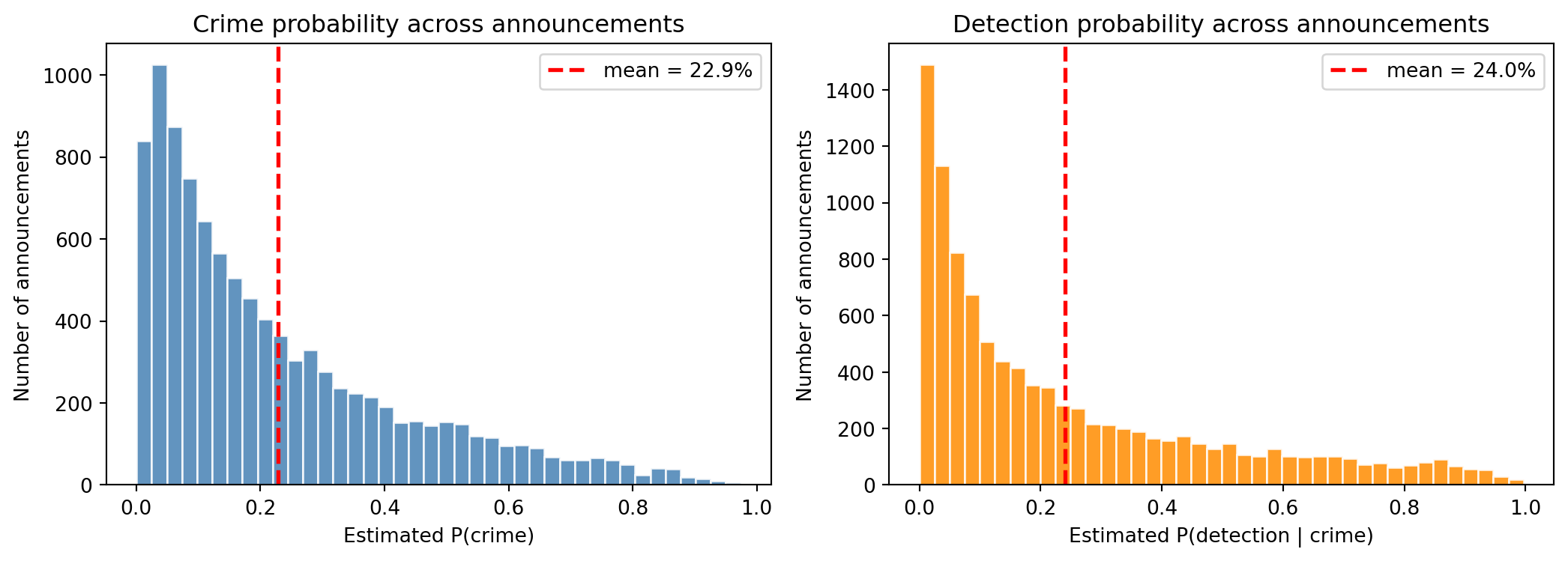
# Top 5 announcements by estimated crime probability
top_crime_idx = np.argsort(p_hat)[::-1][:5]
top_crime_tbl = pd.DataFrame({
    'rank':         range(1, 6),
    'P(crime) est': p_hat[top_crime_idx],
    'info_value':   info_value[top_crime_idx],
    'leakage':      leakage[top_crime_idx],
    'true crime?':  C[top_crime_idx],
    'prosecuted?':  A[top_crime_idx],
})
print('Top 5 announcements by estimated P(crime):')
print(top_crime_tbl.to_string(index=False, float_format='%.2f'))
Top 5 announcements by estimated P(crime):
rank P(crime) est info_value leakage true crime? prosecuted?
1 0.97 3.36 3.90 1 0
2 0.97 3.10 2.77 1 0
3 0.97 2.99 1.99 1 0
4 0.96 2.49 3.23 1 0
5 0.95 3.14 0.79 1 0The top-ranked names have high info_value and leakage, and most of them were crimes in the hidden data, but note that they were mostly not prosecuted.
One caution on interpretation. A high P(detection | crime) score is not an accusation. It means “if a crime had happened here, it would likely be caught”—these are the announcements where surveillance and enforcement are strongest, even though there may be no actual crime at all. Keeping the crime and detection axes separate is the whole reason DCE exists; collapsing them back together at the interpretation stage throws away the identification we are interested in.
When this is less reliable
This synthetic test makes DCE look good for one specific reason: the exclusion restrictions are true by construction. I generated info_value so that it genuinely does not enter the detection equation, and surveillance_signal so that it genuinely does not enter the crime equation.
In real data you have to argue that your crime-only variable really doesn’t affect detection, and vice versa. If you are wrong:
- The prosecution rate may still fit beautifully, because the likelihood only cares about the product
p · d. - But the split between crime and detection can be biased, possibly badly. A misspecified DCE will look fine with the prosecution rate, but wrong with the proportion of total crimes and detection rates.
Three things this synthetic test deliberately does not do, which the real papers do:
Bootstrap confidence intervals. I report Monte Carlo bias and RMSE, how the estimate moves across synthetic worlds. Patel and Putniņš bootstrap samples from a single empirical dataset (1,000 resamples) to get standard errors and intervals.
External validation. Patel and Putniņš go further with validation checks against partially observable real-world truth, informal SEC inquiries, and the out-of-sample test on 724 earnings announcements traded by a group that hacked newswire services. Comerton-Forde and Putniņš add robustness tests and alternative detection specifications, including the distinction between direct and indirect detection.
Argue the instruments. “Detection comes after the trade” is the load-bearing idea. Pre-announcement surveillance signals and regulatory budget can move detection without moving the earlier decision to trade. Whether your instruments satisfy that is an economic argument, not a coding choice.
The bottom line is that the difficulty of estimating the frequency of market crimes lies in whether the variables genuinely separate crime from detection. Get that right, and you can measure a crime rate you never directly observe; get it wrong, and you get a possibly relatively large, biased number. For the fuller treatment—the complete probability matrix, the instrument sets, bootstrap inference, and the validation tests—see the two studies below.
References
Comerton-Forde, C., and Putniņš, T. J. (2014). Stock Price Manipulation: Prevalence and Determinants. Review of Finance 18(1): 23–66.
Feinstein, J. S. (1990). Detection Controlled Estimation. Journal of Law and Economics 33(1): 233–276.
Hansen, B. E. (2022). Econometrics. Princeton University Press.
Morris, T. P., White, I. R., and Crowther, M. J. (2019). Using simulation studies to evaluate statistical methods. Statistics in Medicine 38(11): 2074–2102.
Patel, V., and Putniņš, T. J. (2020). How Much Insider Trading Happens in Stock Markets? Working paper, SSRN 3764192.
Disclaimer: a synthetic illustration of an estimation method, for discussion purposes only. The probabilities recovered here describe data I generated, not any real market or any real party. Not investment advice.