rating difference 0 -> favourite expected to score 0.50
rating difference 50 -> favourite expected to score 0.57
rating difference 100 -> favourite expected to score 0.64
rating difference 200 -> favourite expected to score 0.76
rating difference 400 -> favourite expected to score 0.91Can a chess rating system predict World Cup match winners?
Python
Backtesting
Analysis
Code
At the 2014, 2018 and 2022 World Cups, Elo ratings predicted how often the favourite won, counting a draw as half, to within 3 percentage points.
Elo rates chess players. The same idea applies to football, because the outcomes are the same: win, draw, loss. Each team gets a rating, and the difference between two ratings gives the prediction.
A match gives each team a score of 1 for a win, 0.5 for a draw and 0 for a loss, and Elo turns the rating difference into the favourite’s expected score on the same scale, so the prediction and the result can be compared directly. I compare them at the 2014, 2018, 2022 and 2026 World Cups. At each of them, the favourites’ average expected score is within 0.04 of their average actual score, while picking the favourite as the winner is right in 67 of the 104 matches of 2026, 64%: of the 37 misses, 24 are draws.
The chess method on football
Every team starts on 1500, and two formulas turn each result into a new rating.
First, the rating difference gives the favourite’s expected score, the average score it should take over many such games. The expected score is not the probability of a win: a rating difference of 0 gives each team an expected score of 0.5, its chance of winning plus half its chance of a draw. The expected score is
\[E = \frac{1}{1 + 10^{-\Delta R/400}},\]
where \(\Delta R\) is the favourite’s rating minus the opponent’s before the match, with 65 points added to the home team’s rating unless the ground is neutral, and the 400 sets the scale. Spain on 2000 against Costa Rica on 1600, on neutral ground, have a difference of 400, so Spain’s expected score is \(1/(1 + 10^{-1}) = 0.91\), almost a full win.
Second, the ratings update after the match:
\[R_{\text{new}} = R_{\text{old}} + K\,G\,(S - E),\]
where \(S\) is the actual score on the same 1, 0.5, 0 scale, \(K\) is the weight of the competition, 55 for a World Cup and 20 for a friendly, and \(G\) is a multiplier for the goal margin, 1 for a draw or a one-goal win and larger for a wider win. The two teams’ expected scores add to 1, so one team gains what the other loses: if Spain win this World Cup match by one goal, they gain 55 × (1 − 0.91) ≈ 5 points, and if they lose by one goal, their rating decreases by 55 × 0.91 ≈ 50. A higher K lets one result move a rating further, and the World Football Elo Ratings weight matches from 20 to 60, the range I use. The block below writes the expected-score formula as a function and prints it at five rating differences.
NoteCode: the expected score
def expected_score(rating_difference):
    """The favourite's expected score, from the rating difference in points.

    A difference of 0 gives 0.50, an even game. A difference of 400 gives 0.91, almost a full win.
    """
    return 1 / (1 + 10 ** (-rating_difference / 400))


# The favourite's expected score at a few rating differences.
for rating_difference in (0, 50, 100, 200, 400):
    expected = expected_score(rating_difference)
print(f"rating difference {rating_difference:>4} -> favourite expected to score {expected:.2f}")A 100-point rating difference gives the favourite an expected score of 0.64. So, the lower-rated team is still expected to take 0.36 of the score.
Load the data
Every men’s international with a final score, in date order, from martj42. The final score includes extra time and excludes penalty shootouts, so the code counts a match decided on penalties as a draw, whichever team won the shootout. The neutral flag marks matches on neutral ground, where no home advantage applies.
I do not check this data for accuracy, and I use the file as it is. The block downloads the file each time the page is built, so the match count and the ratings table change as matches are added. Matches played after the 2026 final do not change the World Cup numbers, because the code grades each World Cup match with the ratings from before it.
NoteCode: the matches
import io
import requests
import pandas as pd

url = "https://raw.githubusercontent.com/martj42/international_results/master/results.csv"

# requests brings the file back as one long piece of text. io.StringIO wraps that text so
# that read_csv can treat it as a file, so nothing has to be written to disk first.
response = requests.get(url, timeout=120)
all_matches = pd.read_csv(io.StringIO(response.text))       # the full archive

# Drop every row without a final score, because a match that has not been played can
# teach the ratings nothing.
played_matches = all_matches.dropna(subset=["home_score", "away_score"])
games = played_matches.sort_values("date")                  # oldest first, for the pass below

print("Matches:", f"{len(games):,}", " | through:", games["date"].max())
games.tail(3)[["date", "home_team", "away_team", "home_score", "away_score", "tournament"]]
Matches: 49,945 | through: 2026-10-06| date | home_team | away_team | home_score | away_score | tournament | |
|---|---|---|---|---|---|---|
| 49918 | 2026-10-06 | Algeria | Niger | 2 | 1 | Friendly |
| 49930 | 2026-10-06 | Scotland | Slovenia | 1 | 2 | UEFA Nations League |
| 49944 | 2026-10-06 | Saudi Arabia | United Arab Emirates | 2 | 0 | Gulf Cup |
Build the model
One pass through the archive, oldest first. I save each World Cup rating difference before the result updates the ratings, so no prediction uses the result of its own match. Two adjustments: the home team gets 65 extra rating points unless the ground is neutral, and a win by two or more goals moves the ratings more.
NoteCode: the ratings
START_RATING = 1500.0    # what a team is worth before it has played a match
HOME_ADVANTAGE = 65      # what playing at home is worth, in rating points
WORLD_CUP_YEARS = ("2014", "2018", "2022", "2026")


def match_weight(tournament):
    """K for one match, taken from the name of its tournament.

    'FIFA World Cup' -> 55, 'Friendly' -> 20. The bigger the occasion, the more a single
    result is allowed to move a rating.
    """
    name = tournament.lower()          # lower case first, so the checks ignore capitals
    if "friendly" in name:
        return 20
    if "qualification" in name:
        return 40
    if "world cup" in name or "euro" in name:
        return 55
    continental_cups = ["copa", "african", "asian cup", "gold cup", "nations league"]
    for cup in continental_cups:
        if cup in name:
            return 50
    return 30


def margin_multiplier(goal_margin):
    """How much a wide win counts, as a multiplier on K.

    A draw or a one-goal win counts 1, two goals count 1.5, and above two goals the
    multiplier increases more slowly than the goal margin does.
    """
    if goal_margin <= 1:
        return 1
    if goal_margin == 2:
        return 1.5
    return (11 + goal_margin) / 8


ratings = {}              # team name -> current rating, filled in as teams appear
world_cup_matches = []    # (year, rating_difference, score) for the test below

# to_dict("records") turns the table into a list holding one dictionary per row, so the
# loop reads plain Python dictionaries instead of pandas rows.
for match in games.to_dict("records"):
    home_team = match["home_team"]
    away_team = match["away_team"]

    # .get returns its second argument when the team is not in the dictionary yet, which
    # is how a team that has never played enters on 1500.
    home_rating = ratings.get(home_team, START_RATING)
    away_rating = ratings.get(away_team, START_RATING)

    # str() and upper() read the flag the same way whether the file gives a true or false
    # value or the words themselves.
    neutral = str(match["neutral"]).upper() == "TRUE"
    if neutral:
        home_advantage = 0                                   # neutral ground, so no home advantage
    else:
        home_advantage = HOME_ADVANTAGE
    rating_difference = home_rating - away_rating + home_advantage         # the rating difference the match starts from
    home_expected = expected_score(rating_difference)

    home_goals = int(match["home_score"])
    away_goals = int(match["away_score"])
    if home_goals > away_goals:
        score = 1.0                                     # the chess scale: win, draw, loss
    elif home_goals == away_goals:
        score = 0.5
    else:
        score = 0.0

    # Store the rating difference BEFORE the update, so a prediction never uses its own result.
    year = match["date"][:4]
    if match["tournament"] == "FIFA World Cup" and year in WORLD_CUP_YEARS:
        world_cup_matches.append((year, rating_difference, score))

    margin = abs(home_goals - away_goals)
    k_factor = match_weight(match["tournament"])        # K for this occasion
    move = k_factor * margin_multiplier(margin) * (score - home_expected)
    ratings[home_team] = home_rating + move             # one side gains what the other loses
    ratings[away_team] = away_rating - move

print(f"Trained on {len(games):,} matches and {len(ratings):,} teams. Top of the table:")
rating_table = pd.Series(ratings)                       # keys become labels, values a column
best_first = rating_table.sort_values(ascending=False)
strongest_teams = best_first.head(8)
strongest_teams.round(0)                                # whole rating points are enough
Trained on 49,945 matches and 337 teams. Top of the table:Spain 2352.0
Argentina 2242.0
England 2213.0
France 2181.0
Portugal 2135.0
Brazil 2081.0
Colombia 2068.0
Switzerland 2051.0
dtype: float64Storing the rating difference before the update is the same rule as lagging a signal: Lesson 30 of Python for Investing covers the mistake, and Lesson 20 shows the shift that enforces it in pandas.
How I grade it
The favourite is the team with the higher expected score, home advantage included. Over \(N\) matches in which the favourite wins \(W\) and draws \(D\), I report three rates,
\[\frac{W}{N}, \qquad \frac{W}{N - D}, \qquad \frac{W + 0.5\,D}{N},\]
the favourite’s win rate over all matches, its win rate in decisive matches, those with a winner, and its average actual score. The average actual score is on the same scale as the expected score, so I compare it with the favourite’s average expected score, set before each game. If the two averages are close, the expected scores agree with the actual scores on average over these matches.
NoteCode: the grading
def grade(matches):
    """Score the model on a list of (rating_difference, score) pairs, both read from the home side.

    Returns the counts and the two averages the post reports.
    """
    favourite_wins = 0
    draws = 0
    upsets = 0
    expected_total = 0.0
    actual_total = 0.0

    for rating_difference, score in matches:
        home_expected = expected_score(rating_difference)
        home_is_favourite = home_expected >= 0.5

        # Every number here is written from the favourite's side. When the away team is
        # the higher rated one, both of its numbers are one minus the home team's.
        if home_is_favourite:
            favourite_expected = home_expected
            favourite_actual = score
        else:
            favourite_expected = 1 - home_expected
            favourite_actual = 1 - score
        expected_total += favourite_expected
        actual_total += favourite_actual

        if score == 0.5:
            draws += 1
        elif favourite_actual == 1.0:
            favourite_wins += 1
        else:
            upsets += 1

    number_of_matches = len(matches)
    return {"matches": number_of_matches,
            "favourite_wins": favourite_wins,
            "draws": draws,
            "upsets": upsets,
            "expected": expected_total / number_of_matches,
            "actual": actual_total / number_of_matches}
The 2026 World Cup
I pick the favourite in every 2026 World Cup match.
NoteCode: the 2026 World Cup
def matches_in_year(saved_matches, year_wanted):
    """The (rating_difference, score) pairs from one World Cup.

    Each saved tuple is (year, rating_difference, score), and grade needs only the last two of the three.
    """
    selected = []
    for match_year, match_difference, match_score in saved_matches:
        if match_year == year_wanted:
            selected.append((match_difference, match_score))
    return selected


matches_2026 = matches_in_year(world_cup_matches, "2026")
summary_2026 = grade(matches_2026)

played_2026 = summary_2026["matches"]
wins_2026 = summary_2026["favourite_wins"]
misses_2026 = played_2026 - wins_2026
decisive = wins_2026 + summary_2026["upsets"]   # the decisive matches, which ended with a winner

print(f"Played matches:         {played_2026}")
print(f"Straight winner pick:   {wins_2026}/{played_2026} = {wins_2026 / played_2026:.0%}"
      f"   (a draw counts as a miss)")
print(f"The {misses_2026} misses:          {summary_2026['draws']} draws, "
      f"{summary_2026['upsets']} lost by the favourite")
print(f"On decisive matches:    {wins_2026}/{decisive} = {wins_2026 / decisive:.0%}")
print(f"Expected score {summary_2026['expected']:.2f}  vs  actual {summary_2026['actual']:.2f}"
      f"   (close means the two agree on average)")
Played matches: 104
Straight winner pick: 67/104 = 64% (a draw counts as a miss)
The 37 misses: 24 draws, 13 lost by the favourite
On decisive matches: 67/80 = 84%
Expected score 0.72 vs actual 0.76 (close means the two agree on average)The straight winner pick names the favourite in all 104 matches and is right in 67, 64%. It misses every draw, 24 of its 37 misses, and the favourite lost the other 13. On the 80 decisive matches, the favourite won 67, 84%. The favourite’s average expected score, 0.72, is close to its average actual score, 0.76.
Past World Cups
I grade the three earlier World Cups the same way, with pre-match ratings, and the table reports all four.
NoteCode: the four World Cups
# The same grading as above, once per tournament, collected as one row each.
table_rows = []
for world_cup_year in WORLD_CUP_YEARS:
    tournament_matches = matches_in_year(world_cup_matches, world_cup_year)
    summary = grade(tournament_matches)
    wins = summary["favourite_wins"]
    decisive = wins + summary["upsets"]
    winner_record = f"{wins}/{decisive} = {wins / decisive:.0%}"
    table_rows.append({"World Cup": world_cup_year,
                       "matches": summary["matches"],
                       "winner, decisive": winner_record,
                       "expected score": round(summary["expected"], 2),
                       "actual score": round(summary["actual"], 2)})

pd.DataFrame(table_rows) # a list of dictionaries becomes a table, one row per entry| World Cup | matches | winner, decisive | expected score | actual score | |
|---|---|---|---|---|---|
| 0 | 2014 | 64 | 37/51 = 73% | 0.67 | 0.68 |
| 1 | 2018 | 64 | 36/51 = 71% | 0.68 | 0.66 |
| 2 | 2022 | 64 | 35/49 = 71% | 0.69 | 0.66 |
| 3 | 2026 | 104 | 67/80 = 84% | 0.72 | 0.76 |
The two-decimal averages differ by at most 0.03 in the three earlier tournaments: 0.67 against 0.68 in 2014, 0.68 against 0.66 in 2018, and 0.69 against 0.66 in 2022. In 2026 they differ by 0.04.
One last check, at every level
Errors in opposite directions can cancel in an average over a whole tournament, so I also sort the games into five groups by the favourite’s expected score and plot what each group averaged, one dot per group with its game count. A group whose favourites were expected to score 0.6 should average about 0.6. The grey dashed line marks a perfect match.
NoteCode: the chart
%matplotlib inline
import numpy as np
import matplotlib.pyplot as plt

# One pair per World Cup match, read from the favourite's side: what the model expected
# of it, and what it scored. The chart pools all four tournaments, so the year
# each match belongs to is unpacked but not used.
expected_per_match = []
actual_per_match = []
for match_year, match_difference, match_score in world_cup_matches:
    home_expected_score = expected_score(match_difference)
    if home_expected_score >= 0.5:              # the home team is the favourite, once home advantage is added
        expected_per_match.append(home_expected_score)
        actual_per_match.append(match_score)
    else:
        expected_per_match.append(1 - home_expected_score)
        actual_per_match.append(1 - match_score)

# Both lists become numpy arrays, because an array can be picked over with a list of True
# and False, which is how one group of matches is selected below.
favourite_expected = np.array(expected_per_match)
favourite_actual = np.array(actual_per_match)

group_edges = np.linspace(0.5, 1.0, 6)         # five groups: 0.5 to 0.6, up to 0.9 to 1.0

# digitize says which group each value is in, counting from 1, so subtracting 1 counts
# them from 0. clip folds anything outside the edges into the first or the last group.
group_index = np.clip(np.digitize(favourite_expected, group_edges) - 1, 0, 4)

group_expected = []
group_actual = []
group_sizes = []
for group_number in range(5):
    in_group = group_index == group_number    # True or False for every match
    games_in_group = int(in_group.sum())       # True counts as 1, so the sum is a count
    if games_in_group >= 10:                    # a thinner group averages too roughly
        group_expected.append(favourite_expected[in_group].mean())
        group_actual.append(favourite_actual[in_group].mean())
        group_sizes.append(games_in_group)

RED, TEAL, ORANGE, GREY = "#C0392B", "#17868A", "#D2822B", "#888888"
# The site's chart colours: a cream background, a light grid and a pale frame, so every chart
# on the site has the same look.
BG, INK, GRID, SPINE, AXIS_TEXT = "#FCEFE3", "#1f1f1f", "#EADCCC", "#D5C6B4", "#4a4a4a"


def style_chart(figure, axis):
    """Give a finished chart the site's cream background, light grid and pale frame."""
    figure.patch.set_facecolor(BG)
    axis.set_facecolor(BG)
    axis.grid(True, axis="y", color=GRID, lw=1.0)
    axis.set_axisbelow(True)
    for side in ("top", "right"):
        axis.spines[side].set_visible(False)
    for side in ("left", "bottom"):
        axis.spines[side].set_color(SPINE)
    axis.tick_params(axis="both", length=0, colors=INK, pad=6)
    axis.xaxis.label.set_color(AXIS_TEXT)
    axis.yaxis.label.set_color(AXIS_TEXT)
    axis.title.set_color(INK)
    # Each legend entry in the colour of what it labels: a line's colour or a bar's fill.
    # get_legend() returns None when the chart has no legend.
    legend = axis.get_legend()
    if legend is not None:
        for text, handle in zip(legend.get_texts(), legend.legend_handles):
            if hasattr(handle, "get_color"):
                text.set_color(handle.get_color())
            else:
                text.set_color(handle.get_facecolor())


plt.figure(figsize=(7, 7))
plt.plot([0.5, 1], [0.5, 1], "--", color=GREY, label="perfect match")
plt.plot(group_expected, group_actual, "o-", color=TEAL, lw=2, label="Elo")
for label_x, label_y, label_games in zip(group_expected, group_actual, group_sizes):
    plt.annotate(f"{label_games} games", (label_x, label_y), textcoords="offset points",
                 xytext=(8, -4), fontsize=9, color=GREY)
plt.xlabel("Average expected score of the favourite")
plt.ylabel("Average actual score of the favourite")
plt.title(f"Expected vs actual, four World Cups ({len(world_cup_matches)} games)")
plt.legend(frameon=False)
style_chart(plt.gcf(), plt.gca())       # gcf and gca are the current figure and axis
plt.tight_layout()
plt.savefig("calibration.png", dpi=120, bbox_inches="tight", facecolor=BG)
plt.show()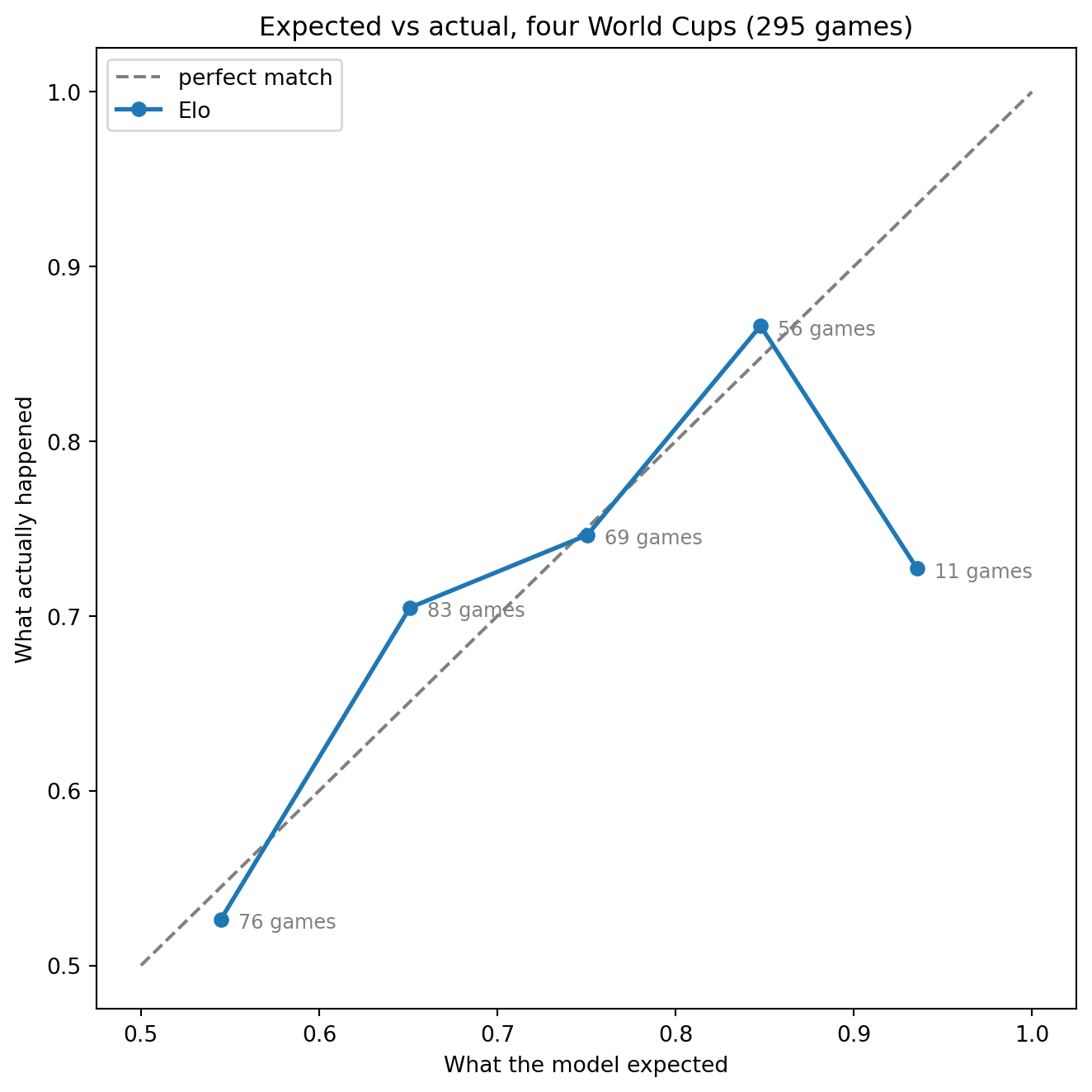
The teal line joins the groups. The four groups from 0.5 to 0.9 are within about 0.06 of the grey dashed line. The top group is below it: its 11 games averaged about 0.73 against an expected score of about 0.94, and with 11 games a single loss in place of a win moves that average by 0.09.
Limitations
A bookmaker’s odds imply separate probabilities of a win, a draw and a loss, and the expected score alone does not supply these three, so it cannot be compared with the odds directly.
Conclusion
The takeaway is that a rating system built for chess, fed only past results, predicted the favourites’ average score at four World Cups to within 0.04, while picking a single winner was right in about two matches in three.
Disclaimer: This post is a teaching example. Not betting advice.