Using the chess rating system to predict the World Cup winners.
Python
Backtesting
Code
A walk-forward test of the chess rating system on four World Cups.
Published
June 30, 2026
Elo rates chess players. The same idea works for football, because the outcomes are the same: win, draw, loss. Each team gets a number, and the gap between two of them is the prediction.
So how well does it call the winners? We test it on four World Cups, 2014 through 2026.
The chess method on football
Every team starts on 1500, and each result moves it. Two formulas.
First, the gap between two ratings gives the favorite’s expected score. A win counts 1, a draw 0.5, a loss 0, and the expected score is the average the favorite should take over many games (nothing to do with goals). Spain on 2000 against Costa Rica on 1600 is a 400-point gap, so Spain’s expected score is 0.91, almost a full win. 0.5 would be a coin flip. It comes from the gap, so it already adjusts for who you played. A plain win rate would not.
expected = 1 / (1 + 10^(-gap / 400))
The 400 just sets the scale. The cell below shows the curve.
Second, the ratings update:
new = old + K * (actual - expected)
actual is what really happened, on that same 1, 0.5, 0 scale. Spain’s and Costa Rica’s expected scores add to 1 (0.91 and 0.09), so one team gains what the other loses.
K is how much a single game can move a rating. A result in line with the prediction moves it little: Spain win as expected and gain about 5 points. The further the result is from the prediction, the larger the move: if Spain lose, they fall about 50. Set K too low and ratings adjust too slowly; too high and a single result moves them too far. The World Football Elo Ratings weight matches from 20 to 60, and we follow that: 55 for a World Cup, 20 for a friendly.
# A feel for the curve: the favorite's expected score at a few rating gaps.for gap in (0, 50, 100, 200, 400): exp =1/ (1+10** (-gap /400))print(f"rating gap {gap:>4} -> favorite expected to score {exp:.2f}")
rating gap    0  ->  favorite expected to score 0.50
rating gap   50  ->  favorite expected to score 0.57
rating gap  100  ->  favorite expected to score 0.64
rating gap  200  ->  favorite expected to score 0.76
rating gap  400  ->  favorite expected to score 0.91
A 100-point lead is worth only 0.64. Clear favorites lose often.
Load the data
Every men’s international with a final score, in date order, from martj42. The neutral flag tells us when home advantage applies.
A quant would usually process this data and check how accurate it is. That is not what this post is about, so we take it as is.
import pandas as pd, requests, iofrom collections import defaultdicturl ="https://raw.githubusercontent.com/martj42/international_results/master/results.csv"games = pd.read_csv(io.StringIO(requests.get(url, timeout=120).text)) # the full archivegames = games.dropna(subset=["home_score", "away_score"]).sort_values("date")print("Matches:", f"{len(games):,}", " | through:", games["date"].max())games.tail(3)[["date", "home_team", "away_team", "home_score", "away_score", "tournament"]]
Matches: 49,519 | through: 2026-07-18
date
home_team
away_team
home_score
away_score
tournament
49516
2026-07-14
France
Spain
0.0
2.0
FIFA World Cup
49517
2026-07-15
England
Argentina
1.0
2.0
FIFA World Cup
49518
2026-07-18
France
England
4.0
6.0
FIFA World Cup
Build the model
One pass through the archive, oldest first. We save each World Cup gap before the result updates the ratings, so no prediction sees its own outcome.
R = defaultdict(lambda: 1500.0) # every team starts at 1500HA =65# home advantage, in rating pointsdef weight(t): # K: how much a result is allowed to move a rating t = t.lower()if"friendly"in t: return20if"qualification"in t: return40if"world cup"in t or"euro"in t: return55return50ifany(w in t for w in ["copa", "african", "asian cup", "gold cup", "nations league"]) else30wc = [] # save World Cup matches for the test belowfor m in games.to_dict("records"): h, a = m["home_team"], m["away_team"] neutral =str(m["neutral"]).upper() =="TRUE" gap = R[h] - R[a] + (0if neutral else HA) # rating gap before the match (home edge unless neutral) exp =1/ (1+10** (-gap /400)) # expected score for the home team (the chess formula) hs, aw =int(m["home_score"]), int(m["away_score"]) score =1.0if hs > aw else (0.5if hs == aw else0.0)if m["tournament"] =="FIFA World Cup"and m["date"][:4] in ("2014", "2018", "2022", "2026"): wc.append((m["date"][:4], gap, score)) # store the gap BEFORE it is updated -> walk-forward margin =abs(hs - aw) g =1if margin <=1else (1.5if margin ==2else (11+ margin) /8) # goal margin, scaled sub-linearly move = weight(m["tournament"]) * g * (score - exp) R[h] += move; R[a] -= moveprint(f"Trained on {len(games):,} matches and {len(R):,} teams. Top of the table:")pd.Series(R).sort_values(ascending=False).head(8).round(0)
Trained on 49,519 matches and 337 teams. Top of the table:
Spain          2293.0
Argentina      2263.0
England        2188.0
France         2138.0
Colombia       2078.0
Brazil         2071.0
Portugal       2062.0
Netherlands    2043.0
dtype: float64
The top of the table is the teams you would expect: Spain, Argentina, France, England, Brazil. No tuning, it falls straight out of the data.
How we grade it
The favorite is the higher-rated team, and the win rate is the percentage of favorites that win. We also compare the favorite’s expected score, set before the game, with what it actually averaged. If the two match, the rating was right.
def grade(rows): # rows = list of (gap, score), score from the home side favw = draws = ups =0; exp_sum = act_sum =0.0; n =len(rows)for gap, score in rows: exp =1/ (1+10** (-gap /400)); fav_home = exp >=0.5 exp_sum += exp if fav_home else1- exp # the favorite's expected score fa = score if fav_home else1- score; act_sum += fa # the favorite's actual scoreif score ==0.5: draws +=1elif fa ==1.0: favw +=1# favorite wonelse: ups +=1# favorite lostreturndict(n=n, favw=favw, draws=draws, upsets=ups, exp=exp_sum/n, act=act_sum/n)
The 2026 World Cup
We pick the higher-rated team in every group game so far.
g = grade([(gap, s) for yr, gap, s in wc if yr =="2026"])dec = g["favw"] + g["upsets"]print(f"Played group matches: {g['n']}")print(f"Straight winner pick: {g['favw']}/{g['n']} = {g['favw']/g['n']:.0%} (a draw counts as a miss)")print(f"The {g['n']-g['favw']} misses: {g['draws']} draws, {g['upsets']} lost by the favorite")print(f"On decisive matches: {g['favw']}/{dec} = {g['favw']/dec:.0%}")print(f"Expected score {g['exp']:.2f} vs actual {g['act']:.2f} (close means the model got it right)")
Played group matches:   103
Straight winner pick:   66/103 = 64%   (a draw counts as a miss)
The 37 misses:          24 draws, 13 lost by the favorite
On decisive matches:    66/79 = 84%
Expected score 0.72  vs  actual 0.76   (close means the model got it right)
The winner rate looks low only because draws count as misses. On games with a winner, the favorite usually won. And the expected score lands almost exactly on the actual.
Past World Cups
2026 is live, so the sample is small. Instead, we can view the three finished World Cups. The ratings are pre-match.
rows = []for yr in ("2014", "2018", "2022", "2026"): g = grade([(gap, s) for y, gap, s in wc if y == yr]); dec = g["favw"] + g["upsets"] rows.append({"World Cup": yr + (""if yr !="2026"else" (so far)"), "matches": g["n"],"winner, decisive": f"{g['favw']}/{dec} = {g['favw']/dec:.0%}","expected score": round(g["exp"], 2), "actual score": round(g["act"], 2)})pd.DataFrame(rows)
World Cup
matches
winner, decisive
expected score
actual score
0
2014
64
37/51 = 73%
0.67
0.68
1
2018
64
36/51 = 71%
0.68
0.66
2
2022
64
35/49 = 71%
0.69
0.66
3
2026 (so far)
103
66/79 = 84%
0.72
0.76
Same every time. Expected and actual are within a hundredth or two: 0.67 vs 0.68 in 2014, 0.68 vs 0.66 in 2018, 0.69 vs 0.66 in 2022. All on games the model never saw.
What it means
Naming the exact winner is only okay, because draws are common and this pick always names a team. But the strength behind it, Elo gets right.
One last check, at every level
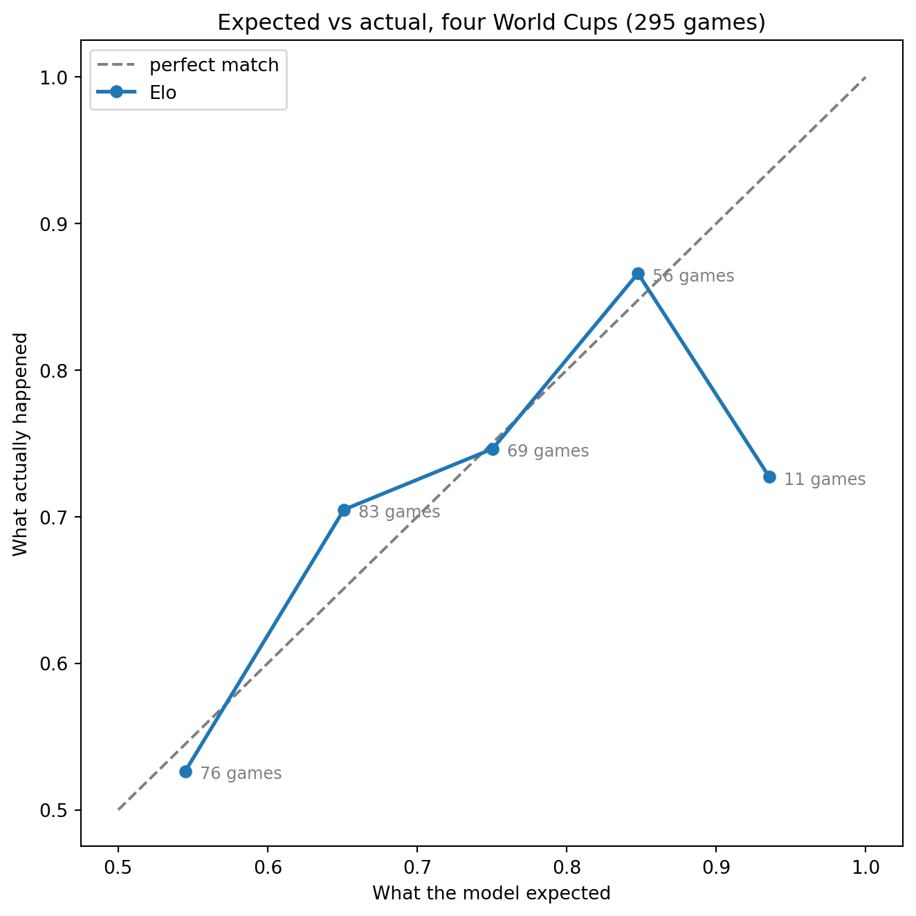
We sort the games by the favorite’s expected score, then plot what each group actually averaged. One dot per group, with its game count. A 0.6 group should average 0.6, a 0.9 group 0.9. The dotted line is a perfect match.
%matplotlib inlineimport numpy as np, matplotlib.pyplot as pltfe = np.array([max(e, 1- e) for e in (1/ (1+10** (-gap /400)) for _, gap, _ in wc)])fa = np.array([(s if (1/ (1+10** (-gap /400))) >=0.5else1- s) for _, gap, s in wc])edges = np.linspace(0.5, 1.0, 6); b = np.clip(np.digitize(fe, edges) -1, 0, 4)xs, ys, ns = [], [], []for k inrange(5): sel = b == kif sel.sum() >=10: xs.append(fe[sel].mean()); ys.append(fa[sel].mean()); ns.append(int(sel.sum()))plt.figure(figsize=(7, 7))plt.plot([0.5, 1], [0.5, 1], "--", color="gray", label="perfect match")plt.plot(xs, ys, "o-", color="#1F77B4", lw=2, label="Elo")for x, y, nn inzip(xs, ys, ns): plt.annotate(f"{nn} games", (x, y), textcoords="offset points", xytext=(8, -4), fontsize=9, color="gray")plt.xlabel("What the model expected"); plt.ylabel("What actually happened")plt.title(f"Expected vs actual, four World Cups ({len(wc)} games)"); plt.legend(); plt.tight_layout()plt.savefig("calibration.png", dpi=120, bbox_inches="tight"); plt.show()
Every dot lands near the line. 0.7 expected, 0.7 actual. 0.9 expected, 0.9 actual. What the model predicts is what happens, so the probabilities hold.
What you do with it
The point is not to perfectly predict who wins but rather to treat the probabilities as scores for “value investing”.
Elo gives a probability, and a bookmaker gives odds, which are a probability with a margin on top. Line the two up, and the difference is the value: if Elo says 60% while the market implies 45%, you are buying a bet that is too cheap, and the rating is what spots it.
The same idea could work for stocks too. Take an earnings announcement, where the reaction on the day often overshoots. But that I leave to the reader.
Disclaimer: This post is a teaching example. Not betting advice.