Following insider trades?
Corporate insiders are officers, directors, and 10 %-plus owners. They are barred from trading on material non-public information. But they can legally trade on everything else—and if anyone knows when their company’s stock is temporarily mispriced, it is them.
Form 4 requires every open-market trade to be reported to the SEC within two business days. OpenInsider, Finviz, and EDGAR let you read the feed in near real time. The question is whether you can build a portfolio that piggybacks on it and beats the index after estimated trading costs.
Lakonishok and Lee (2001) show insider purchases predict returns, especially in small firms. A newsletter that recommended stocks based on insider trades returned 16.0 % annualised against 18.4 % for the S&P over 1985–1997. Klein, Maug, and Schneider (2017) find most insider trades are routine rebalancing, not information-driven. Cohen, Malloy, and Pomorski (2012)—covered in an earlier post—identify the subset of insiders whose trades carry information.
This post tests the naive version: top 50 by net dollar buying, monthly rebalance, estimated trading costs, 2001 to 2026.
The strategy
- All US open-market insider buys and sells on NYSE and Nasdaq. Option exercises, grants, gifts, and tax-withholding trades are excluded—they are mechanical, not discretionary.
- Signal at month
M= net dollar value of insider trades over[M-14, M-3]. The 2-month skip helps reduce look-ahead from late filings and amended Form 4s. - Top 50 stocks by signal, require signal > 0 (net dollar buyer).
- Equal weight, monthly rebalance, intra-month drift.
- Costs: a quote-based half-spread proxy + 0.05 % commission on every rebalance trade—entries, exits, and the trim/top-up trades on survivors whose weights drifted during the month.
- Benchmark: S&P 500, proxied by SPY total return.
Dollar value, not shares. A 1,000-share trade at $1 is not the same signal as 1,000 shares at $500. Ranking on shares gives penny-stock trades the same weight as mega-cap insider purchases, which is wrong.
Starting point
The backtest runs off three in-memory objects. Building them is a separate job that depends on the data vendor. I pull from LSEG Workspace, which is licensed—the raw file and the cleaning logic stay off this page. OpenInsider, Finviz, and EDGAR can replicate the insider-trade feed. The daily return panel and quote-based spread proxy require a separate market-data source such as WRDS or LSEG.
trades—one row per open-market insider trade:Instrument,TransactionDate,Direction('Buy'/'Sell'),SharesTraded,TransactionPrice.daily_wide—Date × Instrumentpanel of daily total returns (decimals).wide_hs—Instrument × monthpanel of the first observed daily half-spread in each month, wherehalf_spread = (Ask - Bid) / (2·Ask). The first-of-month value is a simple proxy for the spread paid at rebalance.
Parameters
The constants used throughout. TOP_N, SIGNAL_LOOKBACK, and SIGNAL_SKIP set the portfolio size and the signal window. COMMISSION and DEFAULT_HS set the cost floor: 0.05 % one-way commission, and a 20 bps half-spread fallback for stocks where the quote panel has no value that month.
import numpy as np
import pandas as pd
import matplotlib.pyplot as plt

TOP_N           = 50      # portfolio size
SIGNAL_LOOKBACK = 12      # months in the signal
SIGNAL_SKIP     = 2       # skip M-1 and M-2 (look-ahead from late filings)
MIN_PERIODS     = SIGNAL_LOOKBACK

COMMISSION = 0.0005       # 0.05 % one-way
DEFAULT_HS = 0.002        # 20 bps fallback half-spread
Step 1. The signal
Sign each trade (+ buy, − sell), multiply by price, aggregate per (stock, month), take a rolling 12-month sum shifted three months back.
trades['TransactionPrice'] = pd.to_numeric(trades['TransactionPrice'], errors='coerce')
trades = trades.dropna(subset=['TransactionPrice']).copy()

trades['trade_value']  = trades['SharesTraded'] * trades['TransactionPrice']
trades['signed_value'] = np.where(trades['Direction'] == 'Buy',
                                   trades['trade_value'],
                                  -trades['trade_value'])
trades['ym'] = trades['TransactionDate'].dt.to_period('M')

monthly_net = (trades.groupby(['Instrument', 'ym'])['signed_value']
                     .sum().reset_index()
                     .rename(columns={'signed_value': 'net_value'}))

wide_net = (monthly_net.pivot(index='Instrument', columns='ym', values='net_value')
                        .fillna(0))
wide_net = wide_net.reindex(sorted(wide_net.columns), axis=1)

# Rolling 12-month sum, shifted by SKIP + 1 months.
# With SIGNAL_SKIP = 2: signal[M] = sum over [M-14, M-3].
rolled      = wide_net.T.rolling(window=SIGNAL_LOOKBACK, min_periods=MIN_PERIODS).sum().T
signal_wide = rolled.shift(SIGNAL_SKIP + 1, axis=1)
The .shift(SIGNAL_SKIP + 1) is the only piece that matters. rolled[M] is the trailing 12-month sum through M, which contains trades filed during M itself and can still get amended. Shifting three months back—excluding M, M-1, M-2—gives a sum over [M-14, M-3], which is safely lagged relative to the M rebalance.
Step 2. The backtest loop
Equal-weight monthly rebalance with three kinds of turnover every month: exits, entries, and the trim/top-up on survivors whose weights drifted. All three cost money. The loop charges for all three.
daily_months = daily_wide.index.to_period('M')

def get_hs(stock, month):
    """Half-spread at rebalance. `wide_hs` stores the first observed daily
    half-spread per (stock, calendar month), so this returns the spread
    quoted on the stock's first trading day of that month."""
    if stock in wide_hs.index and month in wide_hs.columns:
        v = wide_hs.at[stock, month]
        if pd.notna(v):
            return float(v)
    return DEFAULT_HS


def run_backtest(signal_wide):
    rebal = [m for m in signal_wide.columns if signal_wide[m].notna().any()]
    daily_records = []
    prev_holdings = set()
    prev_weights  = {}                          # drifted end-of-prev-month weights

    for m in rebal:
        sig = signal_wide[m].dropna()
        sig = sig[sig > 0]                       # net $-buyers only
        if sig.empty:
            continue

        month_panel = daily_wide.loc[daily_months == m]
        if month_panel.empty:
            continue

        # Eligibility: day-1 return must exist. Checking .notna().all()
        # across the whole month is look-ahead—a delisting with NaN
        # returns after day N would be retroactively dropped, even
        # though live we would have held it on day 1.
        cols = [s for s in sig.index if s in month_panel.columns]
        first_day = month_panel[cols].iloc[0].notna()
        eligible = first_day[first_day].index
        sig = sig.loc[eligible]
        if sig.empty:
            continue

        top        = sig.nlargest(TOP_N).index
        n_held     = len(top)
        tgt_weight = 1.0 / n_held

        # Rebalance cost, survivor-aware.
        # Each stock in prev or new portfolio trades from its drifted
        # weight w_cur to its new target w_tgt. Exits trade down to 0.
        # Entries trade from 0 up to 1/n. Survivors trade from their
        # drifted weight back to 1/n.
        rebal_cost = 0.0
        for s in prev_holdings | set(top):
            w_cur = prev_weights.get(s, 0.0)
            w_tgt = tgt_weight if s in top else 0.0
            trade_size = abs(w_tgt - w_cur)
            if trade_size > 0:
                rebal_cost += trade_size * (get_hs(s, m) + COMMISSION)

        # Monthly rebalance with intra-month drift.
        # Weights set to 1/n on day 1, drift with each stock's
        # cumulative return. The quick version held_panel.mean(axis=1)
        # is equivalent to resetting to 1/n every day—a daily
        # rebalance, not monthly.
        # NaN handling: mid-month missing returns are filled with 0,
        # which holds the stock at its last observed NAV. Whether that
        # captures a delisting loss depends on whether the return field
        # records the final-day write-down.
        held_panel    = month_panel[top].fillna(0.0)
        cum_per_stock = (1 + held_panel).cumprod(axis=0)
        port_nav      = cum_per_stock.mean(axis=1)

        daily_port_ret = port_nav.pct_change()
        daily_port_ret.iloc[0] = port_nav.iloc[0] - 1.0      # day 1: NAV − 1
        daily_port_ret = daily_port_ret.dropna()

        first_idx = daily_port_ret.index[0]
        for date, r in daily_port_ret.items():
            net = r - rebal_cost if date == first_idx else r
            daily_records.append({'Date': date, 'gross': r, 'net': net})

        # Carry drifted end-of-month weights forward.
        final_wealth = cum_per_stock.iloc[-1]
        total_wealth = float(final_wealth.sum())
        prev_weights = (final_wealth / total_wealth).to_dict() if total_wealth > 0 else {}
        prev_holdings = set(top)

    bt = pd.DataFrame(daily_records).set_index('Date').sort_index()
    bt['navs_gross'] = (1 + bt['gross']).cumprod()
    bt['navs_net']   = (1 + bt['net']).cumprod()
    return bt


bt_daily = run_backtest(signal_wide)
Four design choices.
Causal eligibility. iloc[0].notna() uses day 1 only—the information set at rebalance. .notna().all() across the month is look-ahead: it silently drops stocks that delist mid-month.
True monthly rebalance. cum_per_stock.mean(axis=1) on the compounded wealth path gives the NAV of a portfolio set to 1/N on day 1 and left to drift. Taking .mean(axis=1) on the raw daily returns is mathematically identical to resetting to 1/N every day—that is a daily rebalance, not a monthly one.
Survivor-aware costs. Drift pushes winners above 1/N and losers below during the month. Trimming them back costs money. Ignoring that understates trading costs.
Mid-month NaN treatment. fillna(0) holds a stock at its last observed NAV through the end of the month. If the stock posts a crash on its last trading day before delisting, LSEG records it in the total return field and the backtest captures the loss. If the stock simply halts without a final trading day, the residual is not reflected and the position sits at pre-halt NAV until the next rebalance.
Step 3. Benchmark
I proxy the S&P 500 with SPY total return, aligned to the portfolio’s trading days. SPY is the oldest and most liquid S&P 500 ETF, and its auto-adjusted close captures reinvested dividends—close enough to the index for this purpose, and much easier than pulling the index directly. The ten-day leading pad on start is deliberate: without it, pct_change is NaN on the first portfolio day and SPY shifts one day later than the portfolio NAV.
import yfinance as yf

spy = yf.download('SPY',
                  start=str((bt_daily.index.min() - pd.Timedelta(days=10)).date()),
                  end=str((bt_daily.index.max() + pd.Timedelta(days=5)).date()),
                  auto_adjust=True, progress=False)
if isinstance(spy.columns, pd.MultiIndex):
    spy.columns = [c[0] for c in spy.columns]
spy['spy_ret'] = spy['Close'].pct_change()
spy = spy[['spy_ret']].dropna()

common = bt_daily.index.intersection(spy.index)
bt_daily = bt_daily.loc[common].copy()
bt_daily['spy_ret']  = spy.loc[common, 'spy_ret'].values
bt_daily['spy_navs'] = (1 + bt_daily['spy_ret']).cumprod()


def stats(navs, rets):
    n_days = len(navs)
    ann = navs.iloc[-1] ** (252 / n_days) - 1
    vol = rets.std() * np.sqrt(252)
    sr  = ann / vol if vol else np.nan
    return ann, vol, sr

ann_n, vol_n, sr_n = stats(bt_daily['navs_net'], bt_daily['net'])
ann_s, vol_s, sr_s = stats(bt_daily['spy_navs'], bt_daily['spy_ret'])
Step 5. Chart
Two panels. Top: log-scale cumulative NAV. Bottom: rolling 5-year premium.
from matplotlib.lines import Line2D
from matplotlib.ticker import LogLocator, FuncFormatter

INS_COLOR, SP_COLOR = '#1F77B4', '#E67E22'
FILL_INS,  FILL_SP  = '#7FBFDA', '#F0B27A'

fig, (ax1, ax2) = plt.subplots(2, 1, figsize=(14, 11),
                               gridspec_kw={'height_ratios': [3, 2]})
fig.subplots_adjust(hspace=0.30)

# Top panel: cumulative NAV, log scale
ax1.plot(bt_daily.index, bt_daily['spy_navs'], color=SP_COLOR,  lw=2.2)
ax1.plot(bt_daily.index, bt_daily['navs_net'], color=INS_COLOR, lw=2.2)

last = bt_daily.index[-1]
ax1.text(last, bt_daily['spy_navs'].iloc[-1],
         f'  {bt_daily["spy_navs"].iloc[-1]:.1f}x',
         va='center', fontsize=12, fontweight='bold', color=SP_COLOR)
ax1.text(last, bt_daily['navs_net'].iloc[-1],
         f'  {bt_daily["navs_net"].iloc[-1]:.1f}x',
         va='center', fontsize=12, fontweight='bold', color=INS_COLOR)

ax1.set_yscale('log')
ax1.set_ylabel('Cumulative Return (log scale)')
ax1.set_title('Insider portfolio vs S&P 500', fontsize=15, fontweight='bold')
ax1.yaxis.set_major_locator(LogLocator(base=10.0, subs=(1, 2, 3, 5, 7), numticks=20))
ax1.yaxis.set_major_formatter(FuncFormatter(lambda y, _: f'{y:g}x'))
ax1.legend(handles=[
    Line2D([0], [0], color=SP_COLOR,  lw=2.2,
           label=f'S&P 500 ({ann_s:+.1%} ann., SR {sr_s:.2f})'),
    Line2D([0], [0], color=INS_COLOR, lw=2.2,
           label=f'Top-{TOP_N} insider ({ann_n:+.1%} ann., SR {sr_n:.2f})'),
], loc='upper left')
ax1.grid(True, which='both', alpha=0.25)

# Bottom panel: rolling 5-year premium
ax2.fill_between(rolling_ann.index, 0, rolling_ann.values,
                 where=rolling_ann.values >= 0, color=FILL_INS,
                 label='Insider outperforms', interpolate=True)
ax2.fill_between(rolling_ann.index, 0, rolling_ann.values,
                 where=rolling_ann.values < 0, color=FILL_SP,
                 label='S&P 500 outperforms', interpolate=True)
ax2.plot(rolling_ann.index, rolling_ann.values, color='#1a1a1a', lw=1.0)
ax2.axhline(y=0, color='#1a1a1a', lw=0.8)

curr = rolling_ann.iloc[-1]
ax2.text(rolling_ann.index[-1], curr, f'  {curr:+.1f}%',
         va='center', fontsize=12, fontweight='bold',
         color=SP_COLOR if curr < 0 else INS_COLOR)

ax2.set_ylabel('Annualized Premium (%)')
ax2.set_title('Rolling 5-Year Annualized Insider Premium',
              fontsize=13, fontweight='bold')
ax2.legend(loc='upper right')
ax2.grid(True, axis='y', alpha=0.3)

plt.tight_layout()
plt.show()
Results
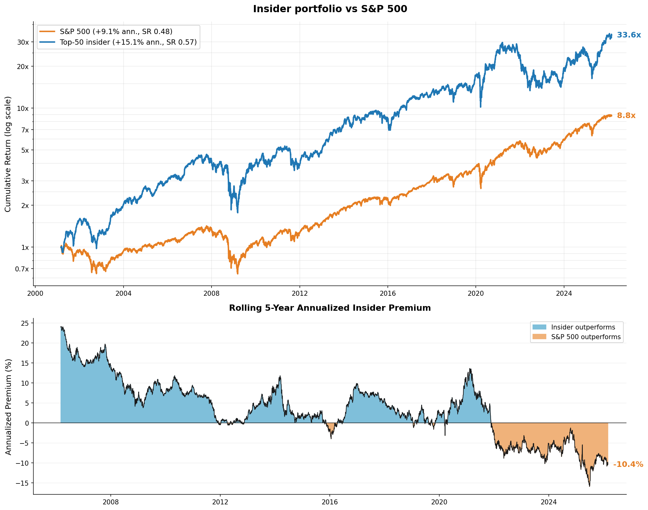
Full sample: 15.1 % annualised vs 9.1 % for the S&P 500, Sharpe 0.57 vs 0.48. A dollar compounded to $33.6 in the portfolio and $8.8 in the index.
But the rolling 5-year premium peaked above 11 % in 2021 and has fallen to −10.4 %. A naive top-50 has lagged the index for about four years.
Three possible explanations for the recent underperformance. Signal decay—more eyes on Form 4 filings through systematic funds means insider news is priced in faster. Regime—insider-heavy portfolios tilt small and value, both of which have trailed mega-cap indices since 2022. Noise—the premium has recovered from comparable drawdowns before.
Whichever it is, this is the naive version. It treats a founder’s opportunistic buy after bad earnings the same as a director’s routine annual top-up. Cohen, Malloy, and Pomorski (2012) argue only the first type is informed; the mechanical trades are noise. Filtering the universe on that dimension is the natural next experiment, and the classifier is in the previous post.
Caveats
Market impact beyond the quoted spread. The cost model charges the half-spread and a commission. Real execution shows slippage past top-of-book, especially in small-caps where this strategy concentrates. Additional slippage beyond the quoted spread is plausible, especially in small-caps
Simultaneous execution at a single price. The backtest assumes all rebalance trades—exits, entries, and survivor trims—fill at the same reference price at the moment of rebalance. In practice, execution has to be sequenced, prices move between fills, and opening and closing auctions are wider than intraday. This is additional slippage on top of the half-spread.
Half-spread measurement itself is noisy. Hagströmer and Hübbert (2026) show conventional trade-quote matching algorithms (Lee–Ready and variants) overstate effective spreads by roughly 8–18 %. A first-day quote as a monthly proxy avoids that trap by not relying on any matching rule—but it is one observation per stock per month, which is its own kind of noise.
Mid-month NaN treatment. fillna(0) holds a stock at its last observed NAV through the end of the month. When a stock posts a crash on its last trading day before delisting, the backtest captures that loss if the total return field records the final-day write-down. When a stock halts and delists without a final trading day — so the last observation is a normal trading day — the residual value is not reflected, and fillna(0) quietly holds the position at pre-halt NAV until the next rebalance. CRSP’s DLRET books the final write-down explicitly; my LSEG pull relies on whatever the feed recorded.
Universe scope. The universe is whatever the LSEG insider pull returns—active and delisted US names over the window. Close to but not identical to Lakonishok and Lee’s full NYSE-AMEX-Nasdaq coverage.
No role filter. Every Form 4 filer—officers, directors, 10 %+ beneficial owners—is kept. Lakonishok and Lee find beneficial-owner trades carry less predictive power than officer and director trades. Dropping them tightens the signal modestly.
References
Cohen, L., Malloy, C., and Pomorski, L. (2012). Decoding Inside Information. Journal of Finance 67(3): 1009–1043.
Hagströmer, B., and Hübbert, A. (2026). Bias in Execution Cost Measures. Working paper, Stockholm Business School.
Klein, O., Maug, E., and Schneider, C. (2017). Trading strategies of corporate insiders. Journal of Financial Markets 34: 48–68.
Lakonishok, J., and Lee, I. (2001). Are Insider Trades Informative? Review of Financial Studies 14(1): 79–111.
Disclaimer: simplified, hypothetical backtest with approximate trading costs for discussion purposes only. Not investment advice. Past performance does not predict future returns.