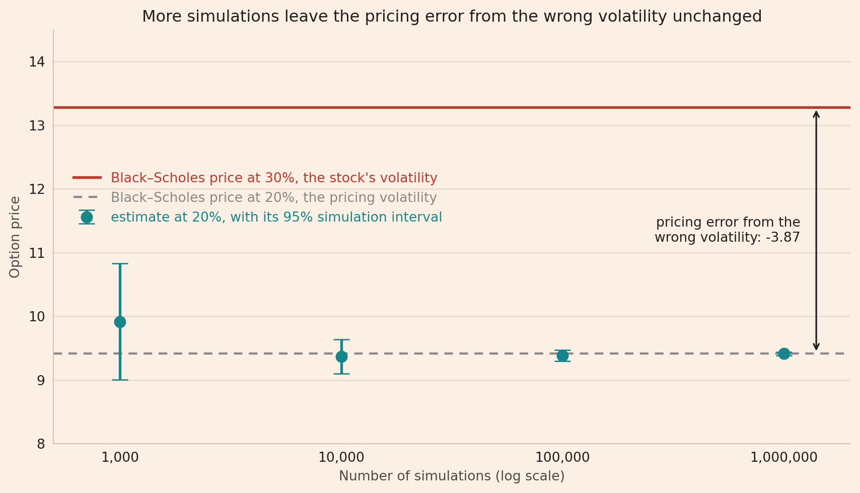
More simulations make an estimated option price more precise, but they leave the error from a wrong volatility input unchanged.
Published
September 23, 2026
A call option gives its holder the right to buy a stock at a fixed price on a set date, the maturity. At maturity, it pays the stock price minus the fixed price when that is positive, and nothing otherwise. The option’s price today is that payoff averaged over the possible stock prices at maturity, weighted by how likely each is under a model of the stock price, and converted into today’s money. For this call, the Black–Scholes formula computes the average exactly. For options without such a formula, such as one that pays according to a stock’s average price over a year, Monte Carlo simulation estimates the price: it draws many stock prices at random, computes each payoff, converts the payoffs into today’s money and averages them.
A simulated price is an estimate, reported with a 95% simulation interval, which measures how much the estimate would change with other random draws, with the model and its inputs unchanged. To test whether a narrow interval means that the price is right, I price a one-year call on a stock that trades at 100, with the right to buy it for 100, by simulation, as if no formula existed, and use the Black–Scholes formula only to check the simulation.
The option’s price depends on the stock’s volatility, how much the stock price will vary over the coming year. Say we estimate the volatility at 20% a year, for example from past stock prices. A million simulated stock prices then give a price of 9.41, with a 95% simulation interval of only 9.39 to 9.44. But in the hypothetical market I construct, which follows the Black–Scholes model, the volatility is in fact 30%, which nobody knows when the option is priced, and at 30% the option is worth 13.28. Trusting the narrow interval, we would wrongly believe that the option is worth about 9.41.
Defining the option and the two volatilities
The option is a European call on one share: the holder can buy the share only on the maturity date, for a fixed price, called the strike, of 100. If the share is worth 120 at maturity, the holder pays 100 for it and can sell it for 120, a payoff of 20. If the share is worth 90, the holder does not buy it, and the payoff is 0. In general, the payoff is
\[\max(S_T - K,\ 0),\]
where \(\max\) takes the larger of the two numbers, \(S_T\) is the stock price at maturity and \(K\) is the strike. As the Black–Scholes formula assumes, the stock pays no dividends, the cash payments that some companies make to their shareholders.
Converting a payoff at maturity into today’s money is called discounting. The risk-free interest rate \(r\), the rate earned on money lent without any risk of loss, is an assumed 3% a year. The rate is continuously compounded, meaning that interest is added at every instant, so an amount grows by the factor \(e^{rT}\) over \(T\) years, where \(e \approx 2.718\) is the base of the natural logarithm. Multiplying a payoff at maturity by \(e^{-rT}\) gives its value today. For one year, \(e^{-0.03} = 0.9704\).
The volatility, \(\sigma\), is the standard deviation (roughly, how far values typically are from their average) of the stock’s annual log return, which the next section defines. I call the 30% that I set for this hypothetical market the stock’s volatility, and the 20% used to price the option the pricing volatility.
Simulating the stock price
The payoff depends only on the stock price at maturity, so each simulation draws that price directly, without simulating the days in between, in two steps:
where \(S_0 = 100\) is the stock price today, \(T = 1\) is the time to maturity in years, \(\sigma = 0.20\) is the pricing volatility, \(r = 0.03\) is the risk-free rate, and \(Z\) is a random draw from the standard normal distribution, the bell-shaped distribution with an average of 0 and a standard deviation of 1. The first step gives the log return \(X_T\), the natural logarithm of the price ratio \(S_T/S_0\), the power to which \(e\) must be raised to give that ratio. Multiplying \(Z\) by \(\sigma\sqrt{T}\) gives the log return’s random part a standard deviation of \(\sigma\sqrt{T}\), and \((r - \sigma^2/2)\,T\) is its average. The second step turns the log return into the stock price at maturity: \(e^{X_T}\) is the ratio \(S_T/S_0\), and multiplying it by \(S_0\) gives \(S_T\).
In the formula, \(\sqrt{T}\) turns the yearly volatility into the volatility over \(T\) years, and \(-\sigma^2/2\) keeps the average stock price the same at any volatility. The rate \(r\) makes the simulated stock grow on average at the risk-free rate: option pricing uses that growth, and that growth is not a forecast of the stock’s return. The box below explains why the formula needs each of the three parts.
NoteWhy the formula has these three parts
The volatility is multiplied by \(\sqrt{T}\) because the log return over \(T\) years is the sum of the log returns of the shorter periods within it. In this model, those log returns are independent, meaning that one period’s log return says nothing about another’s, so their variances, the squares of their standard deviations, add up: \(\sigma^2\) a year gives \(\sigma^2 T\) over \(T\) years, and the standard deviation over \(T\) years is the square root, \(\sigma\sqrt{T}\).
The average of the log return, \((r - \sigma^2/2)\,T\), raises two questions: why the stock grows at the risk-free rate \(r\), and why \(\sigma^2/2\) is subtracted.
The risk-free rate. In the Black–Scholes model, where the stock’s log return is normally distributed with a constant volatility, a portfolio of the stock and a risk-free bond, a loan that earns the rate \(r\), has the same payoff as the option if the number of shares is adjusted at every instant. So the option must cost what that portfolio costs. Otherwise, traders could make a risk-free profit by buying the cheaper of the two and selling the other. That cost does not depend on the stock’s expected growth, so we can price the option as if the stock grew on average at the risk-free rate, which is called risk-neutral pricing. The growth at \(r\) is part of the pricing calculation and is not a forecast of the stock’s return.
The \(-\sigma^2/2\) term. Taking the exponential increases the average: at 20%, the draws \(Z = 1\) and \(Z = -1\) give random parts of 0.20 and −0.20, which average 0, but their exponentials, \(e^{0.20} = 1.22\) and \(e^{-0.20} = 0.82\), average 1.02, above \(e^0 = 1\). Over all standard normal draws, \(e^{\sigma\sqrt{T}Z}\) averages exactly \(e^{\sigma^2 T/2}\), a property of the normal distribution. Subtracting \(\sigma^2 T/2\) in the exponent divides every simulated stock price by this factor, which cancels it, so the average stock price at maturity is \(100 e^{0.03} = 103.05\) at any volatility, today’s price grown at the risk-free rate.
The block below takes two chosen draws, \(Z = 1\) and \(Z = -1\), through the two steps, then computes each payoff and converts it into today’s money.
import numpy as npSTOCK_PRICE =100.0# S0, the stock price todaySTRIKE =100.0# K, the price at which the holder can buy the stock at maturityMATURITY =1.0# T, the time to maturity in yearsRISK_FREE_RATE =0.03# r, the risk-free rate per year, continuously compoundedSTOCK_VOLATILITY =0.30# the stock's volatility, which I set for this hypothetical marketPRICING_VOLATILITY =0.20# the volatility used to price the option# With continuous compounding, 1 paid at maturity is worth exp(-r T) today.DISCOUNT_FACTOR = np.exp(-RISK_FREE_RATE * MATURITY)def stock_price_at_maturity(draw, volatility):"""Turn standard normal draws into stock prices at maturity, at the given volatility. The draw can be one number or a NumPy array of draws, because NumPy applies arithmetic and np.exp to each element of an array. """# exponent is the log return X_T, and np.exp(exponent) is the price ratio S_T / S_0.# ** raises to a power, so volatility**2 is the volatility squared. exponent = ((RISK_FREE_RATE - volatility**2/2) * MATURITY+ volatility * np.sqrt(MATURITY) * draw)return STOCK_PRICE * np.exp(exponent)def discounted_payoff(price_at_maturity):"""Return the call's payoff, max(S_T - K, 0), in today's money. np.maximum takes the larger of each element and 0, so the function takes one price or an array. """ payoff = np.maximum(price_at_maturity - STRIKE, 0.0)return DISCOUNT_FACTOR * payoff# An f-string, f"...", fills in the value of each expression in braces: {x:.4f} writes x with# four decimals, {x:+.0f} with its sign and no decimals, and {x:,} with commas between thousands.print(f"discount factor exp(-rT): {DISCOUNT_FACTOR:.4f}")for draw in [1.0, -1.0]: price_at_maturity = stock_price_at_maturity(draw, PRICING_VOLATILITY) payoff = np.maximum(price_at_maturity - STRIKE, 0.0)print(f"draw {draw:+.0f}: stock price at maturity {price_at_maturity:.2f}, "f"payoff {payoff:.2f}, discounted payoff {discounted_payoff(price_at_maturity):.2f}")
For \(Z = 1\), the log return is \((0.03 - 0.20^2/2) + 0.20 = 0.01 + 0.20 = 0.21\), so the stock price at maturity is \(100 e^{0.21} = 123.37\). The holder pays the strike of 100 for a share worth 123.37, a payoff of 23.37, and discounting converts the payoff into 23.37 × 0.9704 = 22.68 in today’s money. For \(Z = -1\), the log return is 0.01 − 0.20 = −0.19 and the stock price at maturity is \(100 e^{-0.19} = 82.70\), below the strike, so the payoff and the discounted payoff are 0. Each draw gives one discounted payoff, and the estimate of the option’s price averages many of them.
Estimating the price and its 95% simulation interval
The option’s price at 20% is the discounted payoff averaged over all possible draws of \(Z\), each weighted by how likely it is:
where \(\mathrm{E}\), the expected value, is that weighted average. Monte Carlo simulation replaces the expected value with an average over \(n\) independent draws \(Z_1, \dots, Z_n\). Each draw gives a stock price at maturity, and the average of their payoffs, discounted, is the estimate:
where \(S_{T,i}\) is the stock price at maturity that the two steps above give for the draw \(Z_i\), and \(\sum_{i=1}^{n}\) adds up the \(n\) payoffs.
A new set of \(n\) draws would give a different estimate, with the model and its inputs unchanged. The standard error is the standard deviation of the estimate across such repeated sets of draws, and I estimate the standard error from one set of draws:
\[\text{standard error} = \frac{s}{\sqrt{n}},\]
where \(s\) is the standard deviation of the \(n\) discounted payoffs. Dividing by \(\sqrt{n}\) turns the standard deviation of one payoff into the standard deviation of the average of \(n\) payoffs: an average of \(n\) independent values has \(1/n\) of one value’s variance, the square of its standard deviation, and so \(1/\sqrt{n}\) of its standard deviation.
The estimate is an average of many independent payoffs, so it is approximately normally distributed around the option’s price at 20% (the central limit theorem), and a normally distributed value is within 1.96 standard deviations of its average with a probability of 95%. The 95% simulation interval is therefore
and if the \(n\) simulations were repeated many times with new draws, about 95% of these intervals would contain the option’s price at 20%. The interval measures only the variation from the random draws, with the volatility fixed at 20%.
The block below computes the estimate and its interval from 1,000, 10,000, 100,000 and 1,000,000 simulations.
import pandas as pdNUMBERS_OF_SIMULATIONS = [1_000, 10_000, 100_000, 1_000_000] # Python reads 1_000 as 1000Z_95 =1.96# a standard normal draw is between -1.96 and 1.96 with a probability of 95%# rng is NumPy's random number generator. Starting it from a fixed number, the seed 2026,# gives the same draws on every run, so every number in the post reproduces.rng = np.random.default_rng(2026)# Start with an empty list and add one row of results for each number of simulations.rows = []for n_simulations in NUMBERS_OF_SIMULATIONS:# a new set of draws for each number of simulations, one draw per simulation draws = rng.standard_normal(n_simulations) prices_at_maturity = stock_price_at_maturity(draws, PRICING_VOLATILITY) discounted_payoffs = discounted_payoff(prices_at_maturity) estimate = discounted_payoffs.mean()# std() divides the sum of squared deviations from the average by n before the square# root is taken; ddof=1 divides by n - 1 instead, the usual formula for a sample of draws standard_deviation = discounted_payoffs.std(ddof=1) standard_error = standard_deviation / np.sqrt(n_simulations) rows.append({"simulations": n_simulations,"estimate": estimate,"standard deviation of discounted payoffs": standard_deviation,"standard error": standard_error,"interval low": estimate - Z_95 * standard_error,"interval high": estimate + Z_95 * standard_error})results = pd.DataFrame(rows) # each dictionary becomes a row, its keys the column names# index=False leaves out the row numbers, formatters writes the numbers of simulations with# commas, and float_format gives every other number four decimalsprint(results.to_string(index=False, formatters={"simulations": "{:,}".format}, float_format="{:.4f}".format))
simulations  estimate  standard deviation of discounted payoffs  standard error  interval low  interval high
      1,000    9.9160                                   14.7517          0.4665        9.0017        10.8303
     10,000    9.3674                                   13.8442          0.1384        9.0961         9.6388
    100,000    9.3836                                   14.0530          0.0444        9.2965         9.4707
  1,000,000    9.4141                                   14.1347          0.0141        9.3864         9.4418
With 1,000 simulations, the discounted payoffs have a standard deviation of 14.7517, so the standard error is 14.7517/√1,000 = 0.4665. The estimate is 9.9160, and 1.96 standard errors are 1.96 × 0.4665 = 0.9143, so the 95% simulation interval is 9.9160 − 0.9143 = 9.0017 to 9.9160 + 0.9143 = 10.8303.
The standard deviation of the discounted payoffs is between 13.84 and 14.75 at all four numbers of simulations, so each tenfold increase in simulations divides the standard error by roughly \(\sqrt{10} = 3.16\). With a million simulations, the 95% simulation interval is 9.3864 to 9.4418, 0.055 wide.
Computing the Black–Scholes price at 20% and at 30%
At 20%, the Black–Scholes formula checks the simulation, and at 30% it gives the option’s price in this hypothetical market. The formula computes, in order,
where \(N\) is the standard normal distribution function, the probability that a standard normal draw is below a given value. The first term, \(S_0 N(d_1)\), is the value today of the share the holder receives if the option is exercised, meaning used to buy the share. The second term, \(K e^{-rT} N(d_2)\), is the value today of the strike paid then.
The block below computes the Black–Scholes price at 20% and at 30%. For each number of simulations, it then computes the estimate’s simulation error, the estimate minus the Black–Scholes price at 20%, and its total error, the estimate minus the Black–Scholes price at 30%, and checks whether the 95% simulation interval contains each of the two prices: True if it does, False if not.
from scipy.stats import normdef black_scholes_call(volatility):"""Return the Black–Scholes price of the call at the given volatility. norm.cdf is N, the standard normal distribution function: norm.cdf(0) is 0.5. """ d1 = ((np.log(STOCK_PRICE / STRIKE) + (RISK_FREE_RATE + volatility**2/2) * MATURITY)/ (volatility * np.sqrt(MATURITY))) d2 = d1 - volatility * np.sqrt(MATURITY)return STOCK_PRICE * norm.cdf(d1) - STRIKE * DISCOUNT_FACTOR * norm.cdf(d2)black_scholes_price_at_20 = black_scholes_call(PRICING_VOLATILITY)black_scholes_price_at_30 = black_scholes_call(STOCK_VOLATILITY)pricing_error_from_wrong_volatility = black_scholes_price_at_20 - black_scholes_price_at_30print(f"Black–Scholes price at 20%: {black_scholes_price_at_20:.4f}")print(f"Black–Scholes price at 30%: {black_scholes_price_at_30:.4f}")print(f"pricing error from the wrong volatility, the price at 20% minus the price at 30%: "f"{pricing_error_from_wrong_volatility:.4f}\n")# a new table with one row per number of simulations, like resultscomparison = pd.DataFrame({"simulations": results["simulations"]})comparison["simulation error"] = results["estimate"] - black_scholes_price_at_20comparison["total error"] = results["estimate"] - black_scholes_price_at_30# An interval contains a price when its low end is at or below the price and the price is at# or below its high end. & combines two columns of True and False row by row, giving True# where both are True. Python applies & before <=, so each comparison needs its own parentheses.comparison["interval contains price at 20%"] = ( (results["interval low"] <= black_scholes_price_at_20)& (black_scholes_price_at_20 <= results["interval high"]))comparison["interval contains price at 30%"] = ( (results["interval low"] <= black_scholes_price_at_30)& (black_scholes_price_at_30 <= results["interval high"]))print(comparison.to_string(index=False, formatters={"simulations": "{:,}".format}, float_format="{:.4f}".format))
Black–Scholes price at 20%: 9.4134
Black–Scholes price at 30%: 13.2833
pricing error from the wrong volatility, the price at 20% minus the price at 30%: -3.8699

simulations  simulation error  total error  interval contains price at 20%  interval contains price at 30%
      1,000            0.5026      -3.3673                            True                           False
     10,000           -0.0460      -3.9159                            True                           False
    100,000           -0.0298      -3.8997                            True                           False
  1,000,000            0.0007      -3.8692                            True                           False
The Black–Scholes price at 20% is 9.4134. With a million simulations, the interval, 9.3864 to 9.4418, contains 9.4134 and not 13.2833, the price at 30%. At every number of simulations, the interval contains the price at 20% and not the option’s price in this hypothetical market, 13.28.
where \(C_{20\%}\) and \(C_{30\%}\) are the Black–Scholes prices at the two volatilities. The simulation and the formula compute the price at 20% in the same model, so the simulation error comes only from using a finite number of simulations: 0.5026 with 1,000 simulations and 0.0007 with a million. The pricing error from the wrong volatility, 9.4134 − 13.2833 = −3.8699, uses no simulation, so it is the same at every number of simulations. With a million simulations, the total error is 0.0007 − 3.8699 = −3.8692. With 1,000, it is 0.5026 − 3.8699 = −3.3673, smaller in size only because the positive simulation error cancels part of the pricing error. So more simulations make a large simulation error less likely and leave the pricing error from the wrong volatility unchanged.
The chart below plots each estimate at 20% as a teal point with its 95% simulation interval, against the number of simulations on a log scale. The grey dashed line is the Black–Scholes price at 20%, and the red line the price at 30%.
Show the chart code
import matplotlib.pyplot as pltRED, TEAL, GREY ="#C0392B", "#17868A", "#888888"# The site's chart colours, in order: the cream background, the text, the light grid lines,# the pale frame and the axis labels, the same on every chart of the site.BG, INK, GRID, SPINE, AXIS_TEXT ="#FCEFE3", "#1f1f1f", "#EADCCC", "#D5C6B4", "#4a4a4a"def style_chart(figure, axis):"""Give a finished chart the site's cream background, light grid and pale frame.""" figure.patch.set_facecolor(BG) axis.set_facecolor(BG) axis.grid(True, axis="y", color=GRID, lw=1.0) axis.set_axisbelow(True)for side in ("top", "right"): axis.spines[side].set_visible(False)for side in ("left", "bottom"): axis.spines[side].set_color(SPINE) axis.tick_params(axis="both", length=0, colors=INK, pad=6) axis.xaxis.label.set_color(AXIS_TEXT) axis.yaxis.label.set_color(AXIS_TEXT) axis.title.set_color(INK)# Write each legend entry in the colour of what it labels: a line's colour or a bar's fill# colour. get_legend() returns None when the chart has no legend. legend = axis.get_legend()if legend isnotNone:for text, handle inzip(legend.get_texts(), legend.legend_handles):ifhasattr(handle, "get_color"): text.set_color(handle.get_color())else: text.set_color(handle.get_facecolor())# subplots creates the figure and its one chart, axis; figsize is the figure's width and height# in inches.figure, axis = plt.subplots(figsize=(9, 5.2))# axhline draws a horizontal line across the chart at a price, and label is its text in the# legend. lw is the line width and ls the line style: (0, (4, 3)) repeats a dash 4 line widths# long and a gap 3 line widths long, from the start of the line.axis.axhline(black_scholes_price_at_30, color=RED, lw=2.0, label="Black–Scholes price at 30%, the stock's volatility")axis.axhline(black_scholes_price_at_20, color=GREY, lw=1.6, ls=(0, (4, 3)), label="Black–Scholes price at 20%, the pricing volatility")# errorbar draws each estimate as a point with a vertical bar through it. yerr is the distance# from the estimate to either end of the bar, here 1.96 standard errors, so each bar is the# 95% simulation interval. fmt="o" draws the estimates as points, ms sets the points' size and# capsize the width of the short line at each end of a bar.axis.errorbar(results["simulations"], results["estimate"], yerr=Z_95 * results["standard error"], fmt="o", color=TEAL, ms=8, lw=2.0, capsize=6, label="estimate at 20%, with its 95% simulation interval")# annotate() with an empty text draws only an arrow, here with a head at each end, from the# Black–Scholes price at 20% up to the Black–Scholes price at 30%. Its length is the size of the# pricing error from the wrong volatility. It is at 1,400,000 on the horizontal axis, right of# the last estimate.ARROW_POSITION =1_400_000axis.annotate("", xy=(ARROW_POSITION, black_scholes_price_at_30), xytext=(ARROW_POSITION, black_scholes_price_at_20), arrowprops={"arrowstyle": "<->", "color": INK, "lw": 1.2})# The label is centred (va="center") halfway up the arrow, and ha="right" ends the text at 0.85# times the arrow's position, just left of the arrow. \n in the text starts a second line.axis.text(ARROW_POSITION *0.85, (black_scholes_price_at_20 + black_scholes_price_at_30) /2,f"pricing error from the\nwrong volatility: {pricing_error_from_wrong_volatility:.2f}", ha="right", va="center", color=INK)# On a log scale, 1,000, 10,000, 100,000 and 1,000,000 are equally far apart.axis.set_xscale("log")# Mark only the four numbers of simulations on the horizontal axis, written with commas.axis.minorticks_off()axis.set_xticks(NUMBERS_OF_SIMULATIONS)tick_labels = []for n_simulations in NUMBERS_OF_SIMULATIONS: tick_labels.append(f"{n_simulations:,}")axis.set_xticklabels(tick_labels)# the ranges shown on the two axes, with room for the arrow right of the last estimateaxis.set_xlim(500, 2_000_000)axis.set_ylim(8, 14.5)axis.set_xlabel("Number of simulations (log scale)")axis.set_ylabel("Option price")axis.set_title("More simulations leave the pricing error from the wrong volatility unchanged")# frameon=False draws the legend without a box. bbox_to_anchor puts the legend's lower-left# corner at 1% across and 50% up the chart, in the empty space between the widest interval and# the red line.axis.legend(frameon=False, loc="lower left", bbox_to_anchor=(0.01, 0.5))style_chart(figure, axis)# tight_layout() fits the labels inside the figure. savefig writes the chart to a PNG file:# dpi=140 sets its resolution, bbox_inches="tight" trims the empty margin, and facecolor=BG# keeps the cream background. show() displays the chart.plt.tight_layout()plt.savefig("estimates_by_simulations.png", dpi=140, bbox_inches="tight", facecolor=BG)plt.show()
The 95% simulation intervals get shorter around the Black–Scholes price at 20% as the number of simulations increases. The arrow between the two Black–Scholes prices marks the pricing error from the wrong volatility, which has the same size at every number of simulations.
Conclusion
The simulation and the Black–Scholes formula use the same model and the same volatility, 20%, so their agreement checks the simulation and cannot show that 20% is the right volatility. I can compute the pricing error from the wrong volatility only because I set the stock’s volatility in this hypothetical market. For a real option, the volatility input has to be checked on its own, for example by comparing past volatility estimates with the volatility the stock then showed.
The takeaway is that a 95% simulation interval measures only the simulation error, the error from using a finite number of simulations. An estimate computed with the wrong volatility has the same pricing error from the wrong volatility at any number of simulations, so a narrow interval does not show that the price is right.
Disclaimer: a teaching example on simulated data. Not investment advice.