Should you wait for new lows or new highs?
There are two ways to wait. One saver buys only when the market reaches a new low. The other buys only when it reaches a new high. Until then, both leave their monthly savings in cash.
In this post, I measure what each rule costs. I test both on the S&P 500 against a saver who buys every month, across every ten-year saving plan since 1991. For each plan, I report the difference in annual return. The data is licensed, so the pull stays off this page, but every step of the test is here.
Step 1. Three series
We will use three series. First, the S&P 500 price index, because that is the headline index on which new highs and lows are measured. Second is the total-return index, which includes dividends because that is what we actually earn when invested. Third, the 13-week T-bill rate less 0.75 percentage points, a rough proxy for a savings account when not invested in the S&P 500.
Pulling them is a separate job that depends on the data vendor. I pull from LSEG Workspace, which is licensed, so the raw file and the download code stay off this page. Any source with S&P 500 price and total-return history and a short T-bill series will do.
Everything below runs off one in-memory table, d, with one row per calendar month indexed by month:
px—the price index at the month-end close.mkt—the monthly total return, dividends included.rf—the T-bill rate less 0.75 percentage points, as a monthly decimal, lagged one month so the rate is known before it is earned.
The sample runs from February 1988 through June 2026, 461 months. I stop at the last complete month, since a partial month reduced to a month-end value would enter the test as if it were finished. Cash averages 2.38% a year over that span.
Step 2. The structure
The issue is that a new or high depends on one’s own perspective on the horizon. We will consider N different horizons. A new N-month low means this month’s close is the lowest of the last N months. A new N-month high means it is the highest. The current month is included, so at N = 1 every month is both a high and a low. Both rules then buy every month and must match the control exactly.
So, once a month, invested money earns the market return and waiting cash earns the cash rate. This month’s saving then goes into cash. If the rule says buy, the entire cash balance moves into the market.
This rule uses the close of month t and buys at that same close. The money therefore earns its first market return in month t+1.
I test every possible ten-year plan rather than run the test once from 1991 to 2026. In one long run, a krona contributed in 1991 compounds for decades, while one contributed in 2024 barely has time to move. The result would therefore be mostly about the beginning of the sample. With ten-year plans, every starting month gets the same amount of time.
The first plan begins only after the 36-month rule has enough history. This means that a 3-month rule and a 36-month rule are tested over exactly the same months.
import numpy as np                          # arrays and math
import pandas as pd                         # tables and dates

LOOKBACKS = range(1, 37)                    # a new low/high over the last 1 to 36 months
HORIZON   = 120                             # one saving plan is 120 months = 10 years
CONTRIB   = 1.0                             # saved every month; results are per unit contributed

ev = d.index[max(LOOKBACKS):]               # evaluation months, identical for every N
R  = d.loc[ev, "mkt"].to_numpy()            # market returns as a plain fast array
RF = d.loc[ev, "rf"].to_numpy()             # cash returns
N  = len(ev)
STARTS = range(0, N - HORIZON + 1)          # every month a plan could begin

def triggers(n):
    """True where this month's close set a new n-month high / low."""
    p  = d["px"]
    hi = p >= p.rolling(n).max()            # nothing in the last n months was higher
    lo = p <= p.rolling(n).min()
    return hi.loc[ev].to_numpy(), lo.loc[ev].to_numpy()

def run_plan(deploy, s):
    """One saving plan: start at month s, save every month for HORIZON months."""
    invested = cash = 0.0
    for i in range(s, s + HORIZON):
        invested *= 1 + R[i]                # invested money earns the market
        cash     *= 1 + RF[i]               # waiting money earns the deposit rate
        cash     += CONTRIB                 # this month's saving arrives
        if deploy[i]:                       # rule fired: the whole pile goes in
            invested, cash = invested + cash, 0.0
    return invested + cash

print(f"{len(list(STARTS))} plans, first starts {ev[0]}, last ends {ev[-1]}")
306 plans, first starts 1991-02, last ends 2026-06Step 3. From the final pot to an annual return
Money goes in every month, not all at once at the beginning. CAGR assumes one starting amount that is left to grow, so it does not fit this test. I use IRR instead. It is the constant return that would turn the 120 monthly contributions into the final pot. I first find the monthly rate and then convert it to an annual one.
There is no simple formula that gives the rate directly, so I find it by bisection. I start with a low rate and a high rate, test the midpoint, and keep the half that contains the answer. Repeating this narrows the range until only one rate remains.
def irr(final):
    """Annual IRR for a whole array of final pots, by bisection on all of them at once."""
    final  = np.asarray(final, float)
    lo, hi = np.full(final.shape, -0.5), np.full(final.shape, 0.5)   # monthly rates
    for _ in range(60):                                              # 60 halvings is plenty
        mid  = (lo + hi) / 2
        safe = np.where(np.abs(mid) < 1e-12, 1.0, mid)               # avoid dividing by zero
        fv   = np.where(np.abs(mid) < 1e-12, CONTRIB * HORIZON,
                        CONTRIB * ((1 + mid) ** HORIZON - 1) / safe)
        below = fv < final                       # pot is bigger, so the true rate is higher
        lo, hi = np.where(below, mid, lo), np.where(below, hi, mid)
    return (1 + (lo + hi) / 2) ** 12 - 1         # monthly rate to annual

always = np.ones(N, bool)                        # the control: buy every single month
base   = irr([run_plan(always, s) for s in STARTS])

print(f"buying every month: median {np.median(base):.2%} a year, "
      f"worst plan {base.min():.2%}, best {base.max():.2%}")
buying every month: median 10.26% a year, worst plan -7.89%, best 17.49%Buying every month returned a median of 10.26% a year. Depending on the starting month, the annual return ranged from -7.89% to 17.49%. A single long backtest hides that range.
So I compare each rule with the control over the same ten years, plan by plan. For each rule and each N, I take the median of the 306 differences.
Step 4. Every rule, every window, every plan
At N = 1, both rules buy every month and must match the control. The assertion checks that.
rows = []
for n in LOOKBACKS:
    hi_n, lo_n = triggers(n)
    for rule, dep in (("Only at new lows", lo_n), ("Only at new highs", hi_n)):
        gap = (irr([run_plan(dep, s) for s in STARTS]) - base) * 100   # paired, in points
        rows.append({"rule": rule, "n": n,
                     "cost": np.median(gap),          # the typical plan
                     "beat": (gap > 0).mean() * 100}) # share of plans that won

res = pd.DataFrame(rows)
assert np.allclose(res.loc[res.n == 1, "cost"], 0, atol=1e-9), "engine is wrong at n = 1"

print(res.pivot(index="n", columns="rule", values="cost")
         .round(2).loc[[1, 3, 6, 12, 13, 14, 18, 24, 36]].to_string())
rule Only at new highs Only at new lows
n
1 0.00 0.00
3 -0.24 -0.52
6 0.10 -1.00
12 -0.58 -1.67
13 -0.62 -1.67
14 -0.62 -2.98
18 -0.77 -5.12
24 -1.11 -5.58
36 -1.17 -3.85Waiting for lows cost the most. A 12-month low reduced annual return by 1.67 percentage points and did not beat the control in any of the 306 plans. At 24 months, the cost rose to 5.58 points.
Waiting for highs cost much less. A 12-month high reduced annual return by 0.58 points. At six months, the rule added 0.10 points and beat the control in 58% of the plans.
import matplotlib.pyplot as plt

fig, ax = plt.subplots(figsize=(10, 6))
ax.axhline(0, color="#666666", lw=1.2)                    # the control
ax.annotate("buy every month", (36, 0), xytext=(0, 7), textcoords="offset points",
            ha="right", color="#666666")

for rule, colour in (("Only at new lows", "#C44E52"), ("Only at new highs", "#4C72B0")):
    s = res[res.rule == rule].sort_values("n")
    ax.plot(s["n"], s["cost"], "-o", color=colour, lw=2, ms=5, label=rule)

ax.set_xlabel("New high / low over the last N months")
ax.set_ylabel("Difference in annual IRR (percentage points)")
ax.set_title("The price of waiting")
ax.legend(frameon=False, loc="lower left")
ax.grid(color="#dddddd", lw=0.7); ax.set_axisbelow(True)
for side in ("top", "right"):
    ax.spines[side].set_visible(False)

plt.tight_layout(); plt.savefig("price_of_waiting.png", dpi=120, bbox_inches="tight"); plt.show()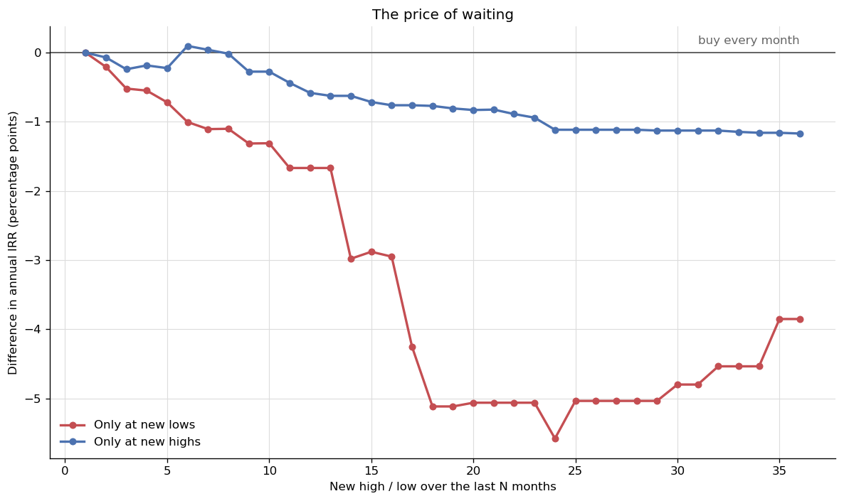
Both lines start at zero, as they should. The high rule stays close to the control and costs at most 1.17 points, at N = 36. The low rule falls slowly through N = 13, then drops.
Step 5. The long waits
Between N = 13 and N = 14, the low rule’s median cost jumps from 1.67 to 2.98 percentage points a year. One extra month adds 1.31 points. To see why, I measure how long the rule can go without buying.
def longest_wait(dep):
    """The longest run of consecutive months in which the rule allowed no purchase."""
    runs, run, start = [], 0, 0
    for i, fired in enumerate(dep):
        if not fired:
            start = i if run == 0 else start
            run += 1
        else:
            if run:
                runs.append((run, ev[start], ev[i - 1]))
            run = 0
    if run:
        runs.append((run, ev[start], ev[-1]))
    return max(runs)

for n in (12, 24):
    hi_n, lo_n = triggers(n)
    for rule, dep in (("low ", lo_n), ("high", hi_n)):
        months, first, last = longest_wait(dep)
        print(f"{n:>2}-month {rule}: {months:>3} months ({months/12:.1f} years) "
              f"with nothing invested, {first} to {last}")
12-month low : 76 months (6.3 years) with nothing invested, 1994-07 to 2000-10
12-month high: 33 months (2.8 years) with nothing invested, 2000-09 to 2003-05
24-month low : 208 months (17.3 years) with nothing invested, 2009-03 to 2026-06
24-month high: 50 months (4.2 years) with nothing invested, 2000-09 to 2004-10A 12-month low rule went 76 months without buying, from July 1994 through October 2000. A 24-month low rule has not bought since March 2009, a stretch of 208 months, or 17.3 years. That is longer than a ten-year plan, so some plans never entered the market.
The 2020 crash did not end the wait. The S&P 500 ended March at 2,584.59, above the December 2018 close of 2,506.85. On monthly data, that was not a new 24-month low. A daily rule would have bought during the crash, but that is a different test.
What this test does not settle
Whether a low is a good price. The test measures what it cost to wait, not whether the low was cheap. It combines the price paid with the time spent in cash and cannot separate the two.
One market, one history. The test covers the S&P 500 over one mostly rising period. That works against a rule that waits for lows. A long falling market could reverse the result. I do not test one.
The fill is idealised. The rule buys at the same close that identifies the new high or low. That price is not known until the close. The test therefore gives the waiting rules a fill they could not know in advance.
The windows overlap. Plans one month apart share 119 of their 120 months. The 306 plans are therefore not 306 independent experiments, and I do not calculate confidence intervals. Ten years is also a choice. A long wait matters more to a five-year saver than a twenty-year one. Nothing is ever sold, and taxes are ignored.
What it means
At almost every N, waiting for a new high or low reduced the median annual return over ten years. The 12-month low rule never beat monthly investing. Apart from N = 1, only the six-month high rule finished ahead, by 0.10 points a year.
The largest costs came when the low rule went years without buying. In this sample, the later purchases did not recover the returns missed while the money waited in cash.
In the end, the simplest rule was hard to beat: invest every month.
Disclaimer: This is a simplified, hypothetical backtest for discussion purposes only, not investment advice. Past performance does not predict future returns.
Data: S&P 500 price and total-return indices and the 13-week Treasury bill, from LSEG Workspace. The pull is licensed and is not reproduced here.