Why a model with no predictive power can score 90% accuracy

When an outcome spans several future observations, training labels can overlap the test period. This post shows how purging that overlap removes the inflated accuracy.

If you are not careful, the way you define your outcome variable can mechanically create look-ahead bias whenever that outcome spans several future days.

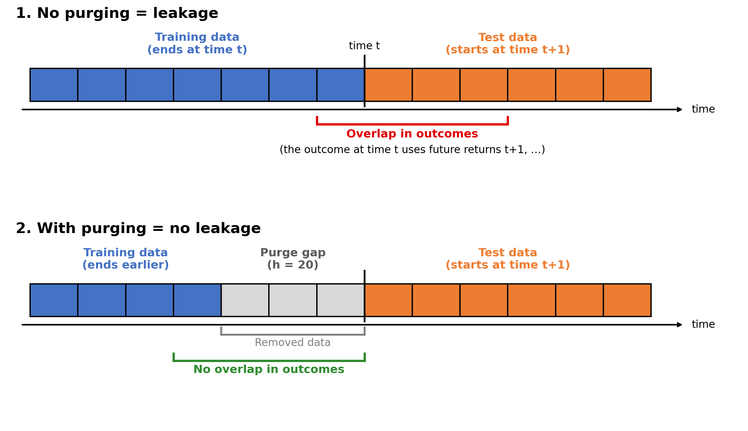
Say the outcome is the cumulative return over the next 20 days. You have 200 days of data and split them in half: training is observations 1 to 100, and test is 101 to 200. Despite it looking good at first, the outcome for training observation 100 is the return over days 101 to 120, which falls within the test set. Every training observation from 81 onward has an outcome that extends beyond day 100 into the test period, so the training outcomes already include test-period returns.

The fix is to purge: drop the training observations near the boundary whose outcomes reach into the test. The picture below shows both cases.

In this post, I will show how this bias inflates a model’s measured accuracy and how that accuracy changes once we correct for it. I simulate a market with no edge, where nothing predicts future returns, and watch a model appear to have a strong edge where none exists. The outcome variable spans 20 future days.

Step 1. A market with no edge

I simulate the returns myself, so we know the truth up front: there is nothing to predict. So, for each day, we simulate returns that are independently drawn from a bell curve centered on zero.

import numpy as np                       # arrays and math
import pandas as pd                      # tables and dates

HORIZON = 20                             # the outcome looks 20 trading days ahead
N       = 6_000                          # how many days we will label
rng     = np.random.default_rng(7)       # a random generator with a fixed seed, so the post reproduces

# We need N days to label, plus HORIZON extra days so the last label still has
# a full 20-day future to look at. That is N + HORIZON returns in total.
dates = pd.bdate_range("2000-01-03", periods=N + HORIZON)          # business days only
ret   = pd.Series(rng.normal(0, 0.01, N + HORIZON), index=dates)  # log returns: mean 0, 1% daily swing

print(f"{len(ret):,} daily log returns, mean {ret.mean():+.5f}, daily vol {ret.std():.4f}")

6,020 daily log returns, mean -0.00013, daily vol 0.0100

Step 2. The outcome: up or down over the next 20 days

The model we will be training will predict whether the next 20 trading days will be up or down. So for each day, I add up the next 20 daily returns and label the day 1 if that sum is positive and 0 if it is not. Because these are log returns, their sum is exactly the 20-day log return.

# rolling(20).sum() adds up each block of 20 days. shift(-20) slides that sum
# back so it lands on the day BEFORE the block, giving each day its "next 20 days".
future = ret.rolling(HORIZON).sum().shift(-HORIZON)   # the 20-day log return that starts tomorrow
y      = (future.iloc[:N] > 0).astype(int).values     # 1 if those 20 days rose, else 0

print(f"{len(y):,} labels, {y.mean():.1%} of them positive")

6,000 labels, 48.4% of them positive

About 48% of the labels are positive, close to the 50% expected from this symmetric simulation. Since future returns are independent of all past information by construction, a valid test should produce accuracy around 50%. The 90.5% result we obtain later therefore cannot represent predictive skill.

Step 3. Two neighbors, almost the same answer

The issue is in the outcome. Each day’s label is built from the 20 returns that follow it, so two days sitting next to each other use almost the same returns. They share 19 of their 20 returns. We can see this directly by lining up two neighboring days.

day = 100                                                  # pick any day and its neighbor
print(f"day {day}'s label uses returns {day + 1} to {day + HORIZON}")
print(f"day {day + 1}'s label uses returns {day + 2} to {day + 1 + HORIZON}")
print(f"the two overlap on returns {day + 2} to {day + HORIZON}: {HORIZON - 1} of {HORIZON}")

day 100's label uses returns 101 to 120
day 101's label uses returns 102 to 121
the two overlap on returns 102 to 120: 19 of 20

Since changing a single term in a sum of twenty barely moves the total, the two labels almost always come out with the same sign. We can confirm this across the whole series:

agree = (y[:-1] == y[1:]).mean()          # how often each label matches the next day's label
print(f"neighboring labels agree {agree:.0%} of the time")

neighboring labels agree 91% of the time

So neighboring labels agree about 91% of the time, and that agreement comes entirely from the overlapping returns. It is worth remembering, because it is what the model will use next.

Step 4. The naive test scores 90%

To test the model, we use walk-forward validation, the standard approach for time series. Instead of a single 50:50 split, we test one day at a time, always training only on the past and then rolling forward. Since training always comes before testing, it may at first appear that there is no way for the model to see the future.

To keep things transparent, I use the simplest setup I can. The only feature is the day’s number, 0, 1, 2, ..., which carries no information about future returns. The model is a one-nearest-neighbor classifier, which means that to label a test day, it finds the single closest training day and copies its answer. Since the feature is just the day number, the closest training day is always the one right before the test day.

from sklearn.model_selection import TimeSeriesSplit      # rolling train/test splits, past before future
from sklearn.neighbors      import KNeighborsClassifier  # the "copy the most similar past day" model
from sklearn.metrics        import accuracy_score        # share of predictions that were correct

X = np.arange(N).reshape(-1, 1)            # the feature: day 0, 1, 2, ... as one column (the shape sklearn wants)

def walk_forward(gap):
    # n_splits=3600 test days; each test set is ONE day; training is up to 252 earlier days (about a year);
    # gap = how many days to drop between the training block and the test day.
    cv = TimeSeriesSplit(n_splits=3_600, test_size=1, max_train_size=252, gap=gap)
    true, pred = [], []
    for train, test in cv.split(X):                       # each loop is one train/test split
        model = KNeighborsClassifier(n_neighbors=1)       # 1 neighbor: copy the single closest day
        model.fit(X[train], y[train])                     # "learn" from the training days
        pred.append(model.predict(X[test])[0])            # predict the one test day
        true.append(y[test][0])                           # keep the correct answer for scoring
    return accuracy_score(true, pred)                     # share the model got right

naive = walk_forward(gap=0)                               # no gap between training and test
print(f"walk-forward, no gap:   {naive:.1%}")

walk-forward, no gap:   90.5%

The model scores 90.5%, even though the feature predicts nothing and the returns contain no signal. A score that high on data with no edge is a clear sign that something has leaked.

Step 5. Look at what the model leaned on

To see where the leak comes from, let us open up the very first split and look at which training day the model actually copied.

def first_split(gap):
    cv = TimeSeriesSplit(n_splits=3_600, test_size=1, max_train_size=252, gap=gap)
    train, test = next(cv.split(X))           # grab just the first (train, test) pair
    last_train  = train[-1]                    # the newest day the model trained on
    test_day    = test[0]                      # the day it must predict
    distance    = test_day - last_train        # how many days apart they are
    shared      = max(HORIZON - distance, 0)   # how many returns their two labels share
    return last_train, test_day, distance, shared

lt, td, dist, shared = first_split(gap=0)
print(f"last training day: {lt}")
print(f"test day:          {td}")
print(f"days apart:        {dist}")
print(f"returns their labels share: {shared} of {HORIZON}")

last training day: 2399
test day:          2400
days apart:        1
returns their labels share: 19 of 20

Now we can see exactly what the model did. The most recent training day is just one day before the test day, so their two labels are built from almost the same returns, sharing 19 of the 20. The model does not have to forecast anything to get the test day right; it can simply copy the answer from the day next door, which is nearly the same. That is why the naive test reaches 90%: it is the same 91% agreement between neighboring days from Step 3, now showing up as accuracy.

Step 6. The fix: purge the overlap

The fix comes straight from the diagnosis: we remove the training days whose outcomes reach into the test. Since the last training day’s outcome reaches 20 days forward, we drop the final 20 training days, the full horizon. Once those are gone, the nearest remaining training outcome ends before the test begins, so the two no longer share any returns. In TimeSeriesSplit, this is a single argument, gap.

lt, td, dist, shared = first_split(gap=HORIZON)           # same inspection, now with the gap
print(f"last training day {lt}, test day {td}, {dist} days apart, labels share {shared} returns")

purged = walk_forward(gap=HORIZON)                        # the only change is the gap
print(f"walk-forward, {HORIZON}-day gap: {purged:.1%}")

last training day 2379, test day 2400, 21 days apart, labels share 0 returns
walk-forward, 20-day gap: 50.3%

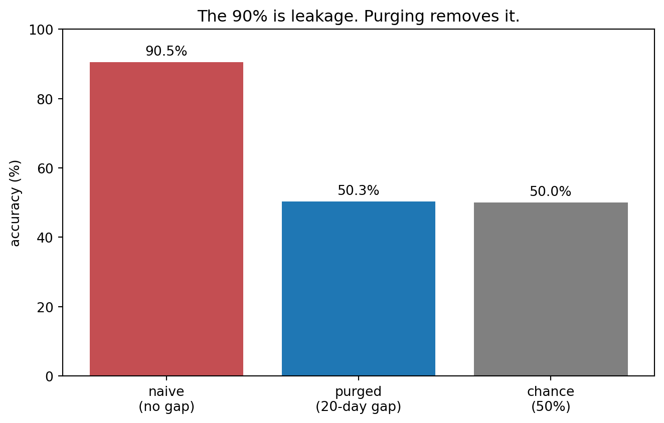
With the gap in place, the nearest training label is now 21 days before the test label and shares none of its returns. Accuracy falls to 50.3%, essentially a coin flip, which is exactly what we should expect when the returns carry no signal. The data, the feature, and the model are all unchanged; the only thing we added was the gap. That single change is enough to make the 90% disappear, because it was leakage all along.

Step 7. The whole picture

Finally, let us put the three numbers side by side: the naive test, the purged test, and the 50% we would expect from chance alone.

import matplotlib.pyplot as plt

# The returns are symmetric around zero, so pure chance is 50%. That is the chance benchmark.
labels = ["naive\n(no gap)", f"purged\n({HORIZON}-day gap)", "chance\n(50%)"]
scores = [naive * 100, purged * 100, 50.0]

plt.figure(figsize=(7, 4.5))
bars = plt.bar(labels, scores, color=["#C44E52", "#1F77B4", "gray"])
plt.ylim(0, 100)                                          # full axis, so the gap is not exaggerated
plt.ylabel("accuracy (%)")
plt.title("The 90% is leakage. Purging removes it.")
plt.bar_label(bars, fmt="%.1f%%", padding=3)              # print each value on top of its bar
plt.tight_layout(); plt.savefig("purging_accuracy.png", dpi=120, bbox_inches="tight"); plt.show()

The purged test returns 50.3% accuracy, close to the 50% expected from the simulated data. The naive test reports 90.5%, so ignoring the label overlap inflates measured accuracy by 40.2 percentage points in this example.

When the horizon is not fixed

In this example, every outcome is exactly 20 days long, so one fixed gap removes all of the overlap at once. In practice, trades are messier because a position can close on a stop-loss, a profit target, or a maximum holding time, so each observation ends up with its own end date. A gap set to the longest possible holding period is still safe, but it throws away more training data than it needs to.

A more precise approach is exact purging, where you drop only the training observations whose outcome windows overlap the test window. When training data also comes after the test block, you purge the overlapping observations there too, and you can add a short embargo, a small gap right after the test period, in case some influence remains longer. This is the general form of purged cross-validation, as set out by López de Prado in Advances in Financial Machine Learning.

What purging does not fix

Accuracy is not profit. Getting the direction right tells us nothing about the size of the gains and losses, or about trading costs, so a strategy can be accurate and still lose money.

The example is extreme on purpose. The day-number feature and the copy-the-neighbor model make the leak unusually large and easy to see, but the underlying problem is general: whenever a training label reaches into the test period, that training row already contains part of the test answer. How much a given model exploits this depends on the labels, features, model, and validation design, and even a two-point overstatement can be enough to pick the wrong model.

Purging only fixes this particular leak. It removes the overlap between training and test outcomes, but other kinds of leakage remain, such as features built from forward-looking windows, a target that peeks ahead, or a scaler fit on the whole sample at once.

Simulated data cannot tell us the size of the effect. It shows the mechanism cleanly, but how large the leak turns out to be in a given dataset is a separate question that depends on the data itself.

What it means

Ordering your data in time is only the first step. Whenever the outcome you are predicting spans several future days, you have to keep the entire outcome window on the correct side of the split, including every future day the label depends on. Otherwise a model that knows nothing can still appear to score 90%, and you will only find out once it fails on genuinely unseen data.

Disclaimer: a teaching example on simulated data. The returns are generated and contain no signal by construction. Not investment advice.

Sources: Marcos López de Prado, Advances in Financial Machine Learning (2018), ch. 7 on cross-validation in finance. Stefan Jansen, Machine Learning for Algorithmic Trading, 2nd ed. (2020), ch. 6 on purging and embargoing. scikit-learn, TimeSeriesSplit.