Are markets overvalued?

Three portfolios’ performance across the full range of S&P 500 monthly returns, 1988 to 2026.

Are markets overvalued? Diversify, and the question matters less.

The valuation debate never ends, and the timing is even harder. So instead of forecasting, I compared how three portfolios performed across the S&P 500’s monthly returns: up months, flat months, and months it fell 10%. The following is the code I used.

The portfolios

Three portfolios, all standard:

• 60/40: 60% stocks, 40% long Treasuries. The default balanced portfolio.
• All Weather: 40% stocks, 30% gold, 30% Treasuries (10% each in 30-, 10-, and 1-year). A simplified version of the Bridgewater idea, holding assets that respond differently to growth and inflation.
• Risk parity: weights set to 1/volatility across stocks, gold, and Treasuries, recomputed each month from trailing data.

The benchmark is 100% stocks, the S&P 500 total-return index.

The setup

• Assets: S&P 500 total return, gold, and 1-, 10-, and 30-year US Treasuries.
• Returns: daily. Rebalance monthly to target weights, then let them drift within the month.
• Two cuts: full-sample risk and return, and each portfolio’s median return across 2.5% windows of the S&P’s monthly return.
• Period: 1988 to 2026. Gross of costs, unlevered.

Median, not mean, for the buckets. The tail buckets are small and skewed, and a single extreme observation can skew the mean too much.

Starting point

The backtest runs off one in-memory object. Building it is a separate job. The download and the cleaning stay off this page; this post is the analysis. The stock series is the same S&P 500 total return I used in an earlier post.

• R: a Date × asset panel of daily total returns for the five building blocks: Stocks (S&P 500 total return), Gold, and three Treasuries T30, T10, T1. 1988 to 2026, one row per trading day, returns in decimals. Days an asset does not trade are filled with a zero return, so the panel keeps one union calendar.

Parameters

import numpy as np
import pandas as pd
import matplotlib.pyplot as plt

VOL_LB_D    = 252           # daily vol lookback for risk parity (~1 year)
ALL_WEATHER = {'Stocks': 0.40, 'Gold': 0.30, 'T30': 0.10, 'T10': 0.10, 'T1': 0.10}
SIXTY40     = {'Stocks': 0.60, 'T30': 0.40}
RP_ASSETS   = ['Stocks', 'Gold', 'T30', 'T10']

Step 1. Build the portfolios

def backtest_drift(Rd, wfunc):
    """Monthly rebalance to target weights, then drift within the month."""
    pm = Rd.index.to_period('M')
    parts = []
    for mth in pd.PeriodIndex(pm.unique()).sort_values():
        idx = Rd.index[pm == mth]
        wt  = wfunc(mth, Rd, pm)
        if wt is None:
            continue
        sub  = Rd.loc[idx, list(wt.index)].fillna(0.0)
        cps  = (1 + sub).cumprod()              # each asset's intra-month wealth path
        navp = (cps * wt.values).sum(axis=1)    # portfolio NAV; weights drift with the path
        dr   = navp.pct_change()
        dr.iloc[0] = float(navp.iloc[0] - 1.0)
        parts.append(dr)
    return pd.concat(parts).sort_index()


def fixed_w(w):
    """Constant target weights every month (60/40, All Weather)."""
    return lambda mth, Rd, pm: pd.Series(w)


def rp_w(mth, Rd, pm):
    """Naive risk parity: weights proportional to 1/vol, from PRIOR months only."""
    prior = Rd.loc[pm < mth, RP_ASSETS]         # strictly before this month (no look-ahead)
    if len(prior) < 21:
        return None
    v  = prior.tail(VOL_LB_D).std()
    v  = v[v > 0].dropna()
    iv = 1.0 / v
    return iv / iv.sum()


res = {
    'Stocks 100%':       backtest_drift(R, fixed_w({'Stocks': 1.0})),
    '60/40':             backtest_drift(R, fixed_w(SIXTY40)),
    'All Weather':       backtest_drift(R, fixed_w(ALL_WEATHER)),
    'Naive risk parity': backtest_drift(R, rp_w),
}

Three design choices.

Drift, not daily reset. Weighting the compounded wealth paths, (cps * wt).sum(axis=1), gives the NAV of a portfolio set to its target weights on day 1 and left to drift. Averaging the raw daily returns instead is mathematically identical to resetting the weights every day. That is a daily rebalance, not a monthly one.

No look-ahead on the weights. rp_w reads pm < mth, strictly the months before this one. January’s risk-parity weights are based on data through December, not January itself.

Equal risk, not equal capital. The inverse-vol weights tilt hard toward the calmest asset. In this sample they land near 18% stocks, 20% gold, 22% 30-year, and 40% 10-year. Treasuries carry the portfolio, which is the point, and also the risk.

Step 2. Full-sample risk and return

Start with what each portfolio earned over the full sample, and at what risk.

def stats(r):
    r    = r.dropna(); n = len(r)
    nav  = (1 + r).cumprod()
    cagr = nav.iloc[-1] ** (252 / n) - 1
    vol  = r.std() * np.sqrt(252)
    sr   = r.mean() / r.std() * np.sqrt(252) if r.std() > 0 else np.nan
    mdd  = float(((nav - nav.cummax()) / nav.cummax()).min())
    return cagr, vol, sr, mdd

Across the full sample, All Weather returned 8.2% annualised and risk parity 6.7%, vs 11.0% for the S&P 500, but at far less risk. The S&P experienced a 55% drawdown with a Sharpe ratio of 0.68; All Weather and risk parity held theirs near 24% with a Sharpe ratio of 0.99. 60/40 sits in between.

Step 3. Performance in each return bucket

The full-sample numbers are averaged across all months. To see how each portfolio performed across the range, I bucket each month by the S&P 500 return into 2.5% windows and take the median return for each portfolio.

from matplotlib.ticker import MultipleLocator
from matplotlib.lines import Line2D

port  = ['60/40', 'All Weather', 'Naive risk parity']
STYLE = {'60/40': ('#009E73', '-.'), 'All Weather': ('#0072B2', '-'),
         'Naive risk parity': ('#D55E00', ':')}
MK    = {'60/40': 'o', 'All Weather': 's', 'Naive risk parity': 'D'}


def to_monthly(s):
    m = (1 + s).resample('ME').prod() - 1
    m.index = m.index.to_period('M')
    return m


M   = pd.concat({k: to_monthly(res[k]) for k in (['Stocks 100%'] + port)}, axis=1).dropna()
spx = M['Stocks 100%'] * 100

centers = [c / 10 for c in range(-100, 101, 25)]   # -10, -7.5, ..., +10  (2.5% windows)
xs, MED = [], {k: [] for k in port}
for c in centers:
    # Bucket CENTRED on c: a month counts if (c-1.25) < S&P return <= (c+1.25).
    # So "-10%" is really -11.25%..-8.75%, a range, not an exact value.
    msk = (spx > c - 1.25) & (spx <= c + 1.25)
    if msk.sum() < 3:
        continue
    xs.append(c)
    for k in port:
        MED[k].append(M[k][msk].median() * 100)

fig, ax = plt.subplots(figsize=(10, 6.2))
ax.plot([min(xs), max(xs)], [min(xs), max(xs)], color='#888', lw=1.7, ls='--')   # S&P, 1:1
for k in port:
    ax.plot(xs, MED[k], marker=MK[k], color=STYLE[k][0], ls=STYLE[k][1], lw=2.6, ms=7)
ax.axhline(0, color='#444', lw=1.3)
ax.axvline(0, color='#bbb', lw=0.9)
ax.xaxis.set_major_locator(MultipleLocator(2.5))
ax.yaxis.set_major_locator(MultipleLocator(2.5))
ax.set_xlim(-11, 11)
ax.set_xlabel('S&P 500 monthly return (%)')
ax.set_ylabel('Median portfolio monthly return (%)')
ax.set_title('Portfolio performance in each S&P 500 monthly-return bucket')
handles = [Line2D([0], [0], color=STYLE[k][0], ls=STYLE[k][1], marker=MK[k], lw=2.6, ms=7, label=k)
           for k in port] + [Line2D([0], [0], color='#888', ls='--', lw=1.7, label='S&P 500 (1:1)')]
ax.legend(handles=handles, loc='upper left')
plt.tight_layout()
plt.show()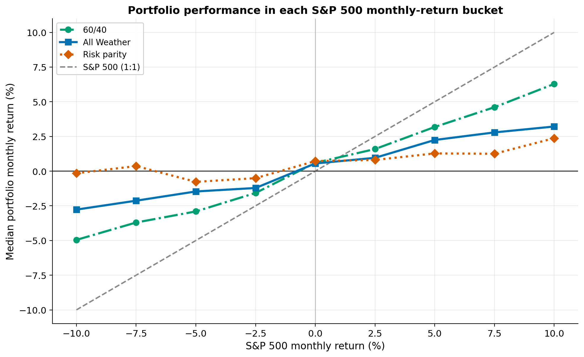

The dashed line is the S&P itself (1:1). Every portfolio line is flatter, because every one holds less in stocks. In the months the S&P fell about 10%, All Weather lost around 3% and risk parity was flat; in the months it rose about 10%, All Weather made about 3% and risk parity about 2%. The flatter the line, the less the portfolio moves with the S&P, in both directions.

Results

The pattern is the same in every bucket: the diversified portfolios move less than the S&P, down and up. That smoother ride costs return. Over the full sample All Weather earned 8.2% a year against 11.0% for the S&P.

This does not mean diversification beats holding stocks in terms of total return. Over this sample it did not. It means the ride is smoother, which is a different thing from a higher return. Whether that trade is worth roughly three points a year is a question about the investor, not the backtest.

Overvalued or not, a sensible allocation cushions you when your forecast is wrong.

Caveats

Gross of costs, unlevered. No commissions, spreads, or rebalancing costs. And risk parity here is unlevered. It is normally run levered to a stock-like volatility, which raises its return and adds financing and margin risk this version ignores.

Buckets are medians. Each point is a median, not a tradeable return, and a bucket is a range rather than a single outcome. The median hides the spread within each bin.

Sample start. The dividend-adjusted S&P 500 total-return series only goes back to 1988, which is why the backtest starts there.

Disclaimer: simplified, hypothetical backtest, gross of costs and unlevered, for discussion purposes only. Not investment advice. Past performance does not predict future returns.