Does a Large One-Day Move in the S&P 500 Predict Next Week’s Return?

One-week S&P 500 total-return outcomes after large single-day moves, 1988 to 2026.

“Buy the dip, sell the rip” is common market advice. On the S&P 500 from 1988 to 2026, it held at the extremes and nowhere else.

After a single day of −5% or worse, the S&P 500 returned a median of +3.81% over the next week. After a day of +5% or better, it returned −1.77%. In the middle, next-week returns sat near zero.

The test is simple. I take every trading day in the S&P 500 Total Return Index from 1988 to 2026, bucket each day by its one-day return, compound the next five trading days, and take the median return in each bucket. That gives one number per bucket: the typical next-week return after a given one-day move.

The setup

• Index: S&P 500 Total Return Index (^SP500TR)
• Period: 1988 to 2026
• Buckets: 1 percentage-point return buckets, with tail buckets at ≤ −5% and ≥ +5%
• Forward window: next 5 trading days
• Statistic: median next-week return

I use the median because the tail buckets are small and skewed. One extreme observation can move the mean too much.

Starting point

The analysis runs off one in-memory object. Building it is a separate job that depends on the data vendor. I pull from LSEG Workspace, which is licensed, so the raw file and the cleaning logic stay off this page. The pipeline is the same one I described in an earlier post, with the universe set to the S&P 500.

• daily, a Series of daily simple returns on the S&P 500 total-return series from 1988 to 2026, indexed by trading day. Total return, so dividends are reinvested back into the index level.

If you do not have an LSEG license, the equivalent open-data path is yfinance with ticker ^SP500TR (the S&P-published total-return index): pull Adj Close, take pct_change(), drop the leading NaN, and the rest of the post runs unchanged.

Parameters

import pandas as pd
import numpy as np
import matplotlib.pyplot as plt

HORIZON_DAYS = 5              # forward window in trading days (~one calendar week)

Step 1. Buckets and the forward-return helper

BUCKETS = [
    ("≤ -5%", -np.inf, -0.050),
    ("-4%",   -0.050, -0.040),
    ("-3%",   -0.040, -0.030),
    ("-2%",   -0.030, -0.020),
    ("-1%",   -0.020, -0.010),
    ("+1%",    0.010,  0.020),
    ("+2%",    0.020,  0.030),
    ("+3%",    0.030,  0.040),
    ("+4%",    0.040,  0.050),
    ("≥ +5%",  0.050,  np.inf),
]


def forward_cum_returns(s, lo, hi, k):
    """Compounded return over the k trading days AFTER each bucket event."""

    # Left tail: exactly as labelled, r <= -5%
    if np.isneginf(lo):
        events = s[s <= hi]

    # Right tail: exactly as labelled, r >= +5%
    elif np.isposinf(hi):
        events = s[s >= lo]

    # Negative interior buckets:
    # (-5%, -4%], (-4%, -3%], ..., (-2%, -1%]
    elif hi <= 0:
        events = s[(s > lo) & (s <= hi)]

    # Positive interior buckets:
    # [+1%, +2%), [+2%, +3%), ..., [+4%, +5%)
    else:
        events = s[(s >= lo) & (s < hi)]

    out = []
    for d in events.index:
        idx = s.index.get_loc(d)
        if idx + k >= len(s):
            continue
        forward = s.iloc[idx + 1: idx + k + 1].values
        out.append(np.prod(1 + forward) - 1)

    return np.array(out)

Two design choices.

Boundary rules. The tail buckets are defined exactly as labelled: returns ≤ −5% go into the left tail, and returns ≥ +5% go into the right tail. The interior negative buckets are defined as (−5%, −4%], (−4%, −3%], …, (−2%, −1%]. The interior positive buckets are defined as [+1%, +2%), [+2%, +3%), …, [+4%, +5%). This assigns every included day to one bucket and avoids double-counting boundary days.

Skip incomplete windows. Events too close to the end of the sample are dropped, so every observation in a bucket has the same forward horizon. Filling forward NaNs with zero would silently bias the recent buckets toward zero.

Slicing from the day after the event is the same discipline as lagging a signal, which Lesson 30 in Learn works through.

Step 2. Aggregate per bucket

rows = []
for label, lo, hi in BUCKETS:
    arr = forward_cum_returns(daily, lo, hi, HORIZON_DAYS)
    rows.append({
        "bucket": label,
        "n": len(arr),
        "median_pct": np.median(arr) * 100 if len(arr) else np.nan,
    })

medians = (pd.DataFrame(rows)
             .set_index("bucket")
             .reindex([b[0] for b in BUCKETS]))

Step 3. Chart

labels = medians.index.tolist()
y_vals = medians["median_pct"].tolist()
x_vals = list(range(len(labels)))
color  = "#d62728"

fig, ax = plt.subplots(figsize=(14, 8))
ax.plot(x_vals, y_vals, "o-", color=color,
        linewidth=2.5, markersize=9, zorder=5)

for xi, yi, lab in zip(x_vals, y_vals, labels):
    offset_y = 14 if yi >= 0 else -16
    ax.annotate(f"{yi:+.2f}%", xy=(xi, yi),
                xytext=(0, offset_y), textcoords="offset points",
                fontsize=10, ha="center",
                va="bottom" if yi >= 0 else "top",
                color=color, fontweight="bold")

ax.axhline(y=0, color="black", linewidth=1.0, zorder=1)
ax.set_xticks(x_vals); ax.set_xticklabels(labels, fontsize=12)
ax.set_xlabel("Single Day Return", fontsize=14)
ax.set_ylabel("One Week Return (%)", fontsize=14)
ax.set_title("One Week After a Single Day Return",
             fontsize=18, fontweight="bold")
ax.grid(True, alpha=0.3)
plt.tight_layout()
plt.show()

Results

Median one-week S&P 500 return after each single-day move bucket, 1988 to 2026. The line rises to +3.81% after days of −5% or worse and falls to −1.77% after days of +5% or better.

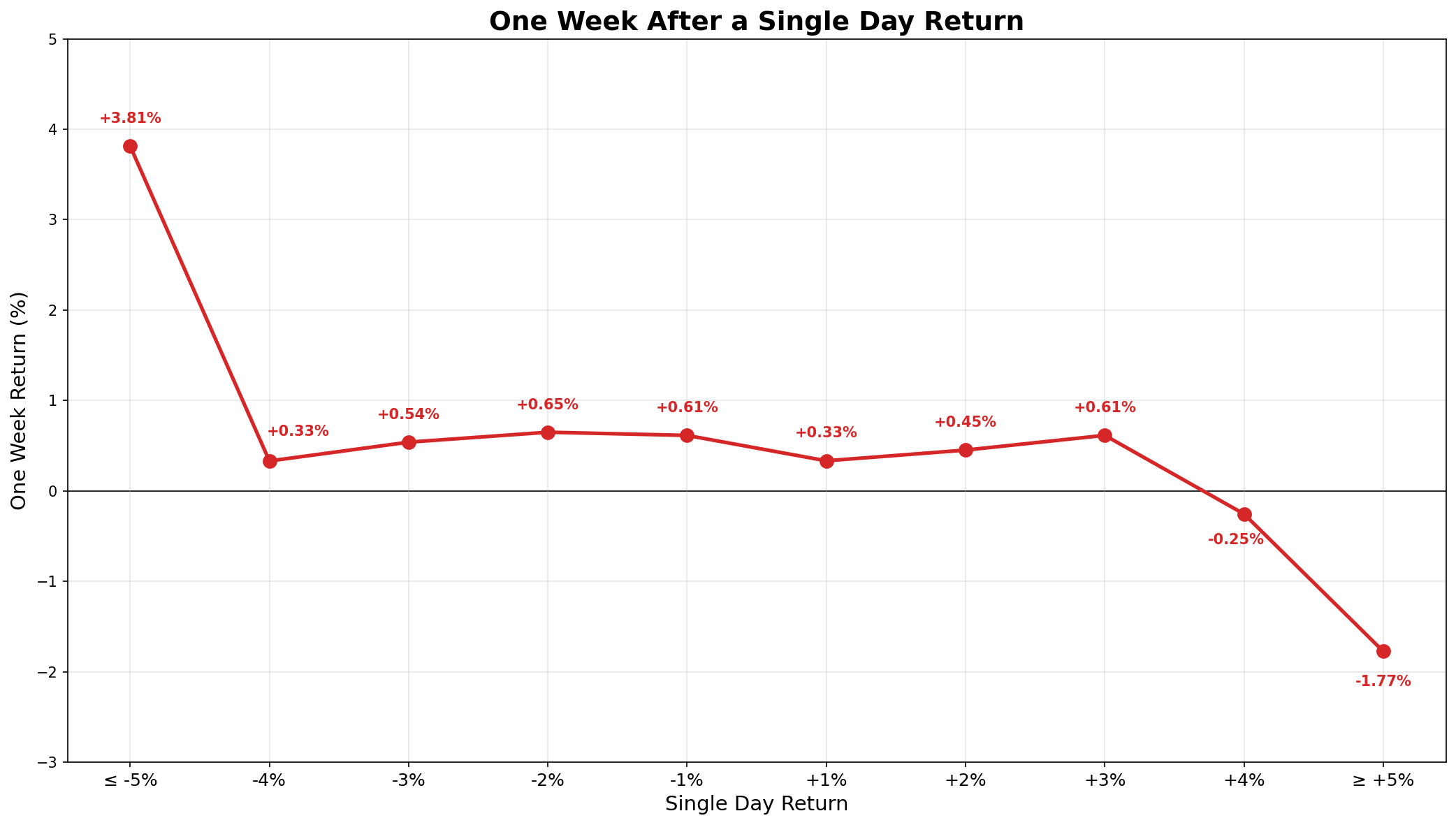
After a ≤ −5% day, the median next-week return is +3.81%.

After a ≥ +5% day, it is −1.77%.

The middle buckets sit close to zero, near the unconditional 5-day forward median of +0.39%.

The signal is at the tails.

At the extremes, the median next-week return moved against the initial one-day move. It is not a signal to buy every large down day or sell every large up day.

Waiting for an extreme day before acting has its own cost, which I measure separately in Should you wait for new lows or new highs?.

The reversal after large down days was larger than after large up days. The extreme buckets are small and cluster in crisis periods, so I do not read much into the gap.

Caveats

Thin tails. The extreme buckets are small. Over 1988 to 2026, the ≤ −5% bucket contains 23 events and the ≥ +5% bucket contains 21. These observations cluster around crisis periods such as 2008 and March 2020. Read the tail estimates as suggestive. Bootstrapping is the way to put a range around a number estimated from this few observations.

Overlapping windows. Large moves often arrive in clusters. If two extreme days occur close together, their next-5-day windows overlap. That means the observations are not fully independent. Purging is what removes that overlap when the same problem shows up in a model.

No execution assumption. This is not a tradable strategy. It does not specify whether the trade happens at the close, the next open, or some other price. It also ignores spreads, slippage, and implementation.

Not a strategy return. The chart shows the median next-week return conditional on the previous day’s move. It does not show the return from a portfolio rule. A rule that only trades after ±5% days would trade very rarely. Turning a rule like this into a tested strategy, with costs, is the subject of How to backtest a strategy.

One index, one sample. The result is for the S&P 500 Total Return Index from 1988 to 2026. Other markets, other horizons, or other samples may look different.

Data source

S&P 500 Total Return Index, pulled from LSEG Workspace (licensed). Dividend reinvestment is built into the index level itself, so the daily simple return from pct_change() reflects a reinvesting investor. The download pipeline is in an earlier post. Free equivalent: Yahoo’s ^SP500TR via yfinance.

Read next

• Should you wait for new lows or new highs? The other side of the same question. What waiting for a signal cost a monthly saver over ten years.
• Why you need to bootstrap your trading strategy The tool for the thin-tail problem above: a confidence range around a number built from few observations.
• Why a model with no predictive power can score 90% accuracy What overlapping windows do to a model, and how purging removes it.
• How to backtest a strategy Turning a rule into a tested strategy, in a few lines, with costs.

If you want to run this yourself and are starting from scratch, Learn goes from variables and prices through to a working backtest in 38 lessons.

Disclaimer: hypothetical analysis on a historical total-return series, for discussion purposes only. Not investment advice. Past performance does not predict future returns.