Investing in high-yield dividend stocks?

Investors like stocks that pay dividends. I would bet there are more books on dividend investing than on any other equity strategy.
But a dividend is just cash leaving the company. It does not create value on its own. The share price often marks down by the dividend amount on the ex-date. But does buying the highest-yielding stocks beat the market anyway?
This test is simple. Build a top-30 portfolio by trailing dividend yield, rebalance monthly with estimated trading costs, and compare to the S&P 500 from 2011 to 2026.
The setup
- Universe: US common stocks on NYSE and Nasdaq, active and delisted.
- Signal at month
M= last observed dividend yield strictly before the first trading day ofM, ffilled per stock. - Top 30 by yield, with yield in
(0%, 30%], last observation within 365 days, market cap above $500m. Skip the rebalance if fewer than 25 qualify. - Equal weight, monthly rebalance, intra-month drift.
- Costs: bid-ask half-spread on the rebalance day + 0.05% commission, applied to every trade — entries, exits, and the trim/top-up trades on survivors whose weights drifted.
- Benchmark: S&P 500, proxied by SPY total return.
- Period: 2011 to 2026.
Yield, not absolute payout. A $1 annual dividend on a $20 stock is a different signal from a $1 dividend on a $200 stock. Ranking on yield is the standard convention.
Starting point
The backtest runs off five in-memory objects. Building them is a separate job that depends on the data vendor. I pull from LSEG Workspace, which is licensed—the raw file and the cleaning logic stay off this page. The pipeline is the same one I described in an earlier post, with the universe set to all US common stocks on NYSE and Nasdaq.
daily_wide—Date × Instrumentpanel of daily total returns (decimals).wide_yield_daily—Date × Instrumentpanel of dividend yields in percent, forward-filled per stock through time.wide_yield_obsdate—parallel panel storing the date of each cell’s most recent yield observation. Used by the freshness filter.wide_mc_daily—Date × Instrumentpanel of company market cap in USD millions, forward-filled.wide_hs_daily—Date × Instrumentpanel of the daily half-spread(Ask − Bid) / (2·Ask). Not ffilled.
Parameters
import numpy as np
import pandas as pd
import matplotlib.pyplot as plt

TOP_N               = 30        # portfolio size
MIN_HOLDINGS        = 25        # require at least this many qualifying names — skip otherwise
MIN_YIELD           = 0.0       # exclusive lower bound (must pay a dividend)
MAX_YIELD           = 30.0      # upper cap in percent (filters distressed / data errors)
MAX_SIGNAL_AGE_DAYS = 365       # drop stocks whose last yield observation is older than this
MIN_MARKET_CAP_M    = 500       # USD millions — size floor at signal_date

COMMISSION = 0.0005             # 0.05 % one-way
DEFAULT_HS = 0.002              # 20 bps fallback half-spread

daily_months = daily_wide.index.to_period('M')
Step 1. Pick the top 30 each month
def pick_top_n(signal_date, rebal_date):
    """Top-N by dividend yield at signal_date, with freshness, market-cap,
    and eligibility filters. Returns None if fewer than MIN_HOLDINGS qualify."""

    sig = wide_yield_daily.loc[signal_date].dropna()
    sig = sig[(sig > MIN_YIELD) & (sig <= MAX_YIELD)]

    # Freshness: drop stocks whose last yield observation is older than the cap.
    obs_dates = pd.to_datetime(
        wide_yield_obsdate.loc[signal_date].reindex(sig.index),
        errors='coerce')
    age_days = (signal_date - obs_dates).dt.days
    sig = sig[age_days <= MAX_SIGNAL_AGE_DAYS]

    # Market-cap floor at signal_date.
    mc = pd.to_numeric(
        wide_mc_daily.loc[signal_date].reindex(sig.index),
        errors='coerce')
    sig = sig[mc >= MIN_MARKET_CAP_M]

    # Eligibility: the stock must have a return on the actual rebalance day.
    month_panel = daily_wide.loc[daily_months == rebal_date.to_period('M')]
    cols = [s for s in sig.index if s in month_panel.columns]
    first_day_has = month_panel[cols].iloc[0].notna()
    sig = sig.loc[first_day_has[first_day_has].index]

    if len(sig) < MIN_HOLDINGS:
        return None

    return sig.nlargest(TOP_N).index
Three design choices.
No look-ahead on the yield. The signal is the yield before the rebalance day, not the first yield observation in the rebalance month. Using “first observation in month M” would be look-ahead: if a stock’s first January yield update arrives on Jan 17, that value cannot be used to pick the stock at the Jan 2 open. The ffilled panel solves this — at every date it stores the last yield known as of that date.
Freshness cap. Forward-filling has no time limit by default. A delisted name’s last yield from two years ago would still rank if we never looked. The freshness filter requires the last yield observation to be within 365 days of the signal date.
Market-cap floor. Pure yield ranking is dominated by microcaps whose yield = dividend / price has shot up because the price collapsed. The $500m floor drops the worst of this.
Step 2. The backtest loop
def get_hs(stock, rebal_date):
    """Half-spread observed on rebal_date itself. Falls back to DEFAULT_HS
    when no quote was recorded that day, rather than a stale spread."""
    if stock in wide_hs_daily.columns and rebal_date in wide_hs_daily.index:
        v = wide_hs_daily.at[rebal_date, stock]
        if pd.notna(v):
            return float(v)
    return DEFAULT_HS


def run_backtest():
    rebal_months = sorted(daily_months.unique())
    daily_records = []
    prev_holdings = set()
    prev_weights  = {}                          # drifted end-of-prev-month weights

    for m in rebal_months:
        month_panel = daily_wide.loc[daily_months == m]
        if month_panel.empty:
            continue
        rebal_date = month_panel.index[0]

        # signal_date = last trading day strictly before rebal_date
        pos = wide_yield_daily.index.searchsorted(rebal_date) - 1
        if pos < 0:
            continue
        signal_date = wide_yield_daily.index[pos]

        top = pick_top_n(signal_date, rebal_date)
        if top is None:
            continue                            # below MIN_HOLDINGS — skip rebalance

        n_held     = len(top)
        tgt_weight = 1.0 / n_held

        # Rebalance cost, survivor-aware.
        # Each stock in prev or new portfolio trades from its drifted
        # weight w_cur to its new target w_tgt. Exits trade down to 0.
        # Entries trade from 0 up to 1/n. Survivors trade from their
        # drifted weight back to 1/n.
        rebal_cost = 0.0
        for s in prev_holdings | set(top):
            w_cur = prev_weights.get(s, 0.0)
            w_tgt = tgt_weight if s in top else 0.0
            trade = abs(w_tgt - w_cur)
            if trade > 0:
                rebal_cost += trade * (get_hs(s, rebal_date) + COMMISSION)

        # Monthly rebalance with intra-month drift.
        # Weights set to 1/n on day 1, drift with each stock's cumulative
        # return. The quick version held_panel.mean(axis=1) on raw returns
        # is equivalent to resetting to 1/n every day — a daily rebalance,
        # not monthly.
        held_panel    = month_panel[top].fillna(0.0)
        cum_per_stock = (1 + held_panel).cumprod(axis=0)
        port_nav      = cum_per_stock.mean(axis=1)

        daily_port_ret = port_nav.pct_change()
        daily_port_ret.iloc[0] = port_nav.iloc[0] - 1.0      # day 1: NAV − 1
        daily_port_ret = daily_port_ret.dropna()

        first_idx = daily_port_ret.index[0]
        for date, r in daily_port_ret.items():
            net = r - rebal_cost if date == first_idx else r
            daily_records.append({'Date': date, 'gross': r, 'net': net})

        # Carry drifted end-of-month weights forward.
        final_wealth = cum_per_stock.iloc[-1]
        total_wealth = float(final_wealth.sum())
        prev_weights = (final_wealth / total_wealth).to_dict() if total_wealth > 0 else {}
        prev_holdings = set(top)

    bt = pd.DataFrame(daily_records).set_index('Date').sort_index()
    bt['navs_gross'] = (1 + bt['gross']).cumprod()
    bt['navs_net']   = (1 + bt['net']).cumprod()
    return bt


bt_daily = run_backtest()
Four design choices.
Causal eligibility. The first_day_has check inside pick_top_n uses the first trading day of the month only — the information set at rebalance. .notna().all() across the whole month would be look-ahead: it silently drops stocks that delist mid-month.
True monthly rebalance. cum_per_stock.mean(axis=1) on the compounded wealth path gives the NAV of a portfolio set to 1/N on day 1 and left to drift. Taking .mean(axis=1) on the raw daily returns is mathematically identical to resetting to 1/N every day — that is a daily rebalance, not a monthly one.
Survivor-aware costs. Drift pushes winners above 1/N and losers below during the month. Trimming them back at rebalance costs money on every survivor, not just on the names entering or exiting. With 30 names and ~5 turnover per month, that is 25 survivor trades on top of 5 exits and 5 entries.
Mid-month NaN treatment. fillna(0) holds a stock at its last observed NAV through the end of the month. If the stock posts a crash on its last trading day before delisting, LSEG records it in the total return field and the backtest captures the loss. If the stock halts without a final trading day, the residual is not reflected and the position sits at pre-halt NAV until the next rebalance.
Step 3. Benchmark and chart
For this post, we can use SPY total return as the S&P proxy, aligned to portfolio trading days. We can use Yahoo Finance to download SPY and then annualize the stats, and later use the rolling 5-year geometric premium for the bottom panel.
import yfinance as yf
from matplotlib.lines import Line2D
from matplotlib.ticker import LogLocator, FuncFormatter

# SPY benchmark
spy = yf.download('SPY',
                  start=str((bt_daily.index.min() - pd.Timedelta(days=10)).date()),
                  end=str((bt_daily.index.max() + pd.Timedelta(days=5)).date()),
                  auto_adjust=True, progress=False)
if isinstance(spy.columns, pd.MultiIndex):
    spy.columns = [c[0] for c in spy.columns]
spy['spy_ret'] = spy['Close'].pct_change()
spy = spy[['spy_ret']].dropna()

common = bt_daily.index.intersection(spy.index)
bt_daily = bt_daily.loc[common].copy()
bt_daily['spy_ret']  = spy.loc[common, 'spy_ret'].values
bt_daily['spy_navs'] = (1 + bt_daily['spy_ret']).cumprod()


# Annualised stats
def stats(navs, rets):
    n_days = len(navs)
    ann = navs.iloc[-1] ** (252 / n_days) - 1
    vol = rets.std() * np.sqrt(252)
    sr  = ann / vol if vol else np.nan
    return ann, vol, sr

ann_n, vol_n, sr_n = stats(bt_daily['navs_net'], bt_daily['net'])
ann_s, vol_s, sr_s = stats(bt_daily['spy_navs'], bt_daily['spy_ret'])

# Rolling 5-year premium (geometric, compounded separately)
ROLL_DAYS = 252 * 5
port_cum  = ((1 + bt_daily['net']).rolling(ROLL_DAYS)
             .apply(lambda x: x.prod(), raw=True))
spy_cum   = ((1 + bt_daily['spy_ret']).rolling(ROLL_DAYS)
             .apply(lambda x: x.prod(), raw=True))
port_cagr = port_cum ** (252 / ROLL_DAYS) - 1
spy_cagr  = spy_cum  ** (252 / ROLL_DAYS) - 1
rolling_ann = ((port_cagr - spy_cagr) * 100).dropna()

# Two-panel chart
DIV_COLOR, SP_COLOR = '#1F77B4', '#E67E22'
FILL_DIV,  FILL_SP  = '#7FBFDA', '#F0B27A'

fig, (ax1, ax2) = plt.subplots(2, 1, figsize=(14, 11),
                               gridspec_kw={'height_ratios': [3, 2]})
fig.subplots_adjust(hspace=0.30)

ax1.plot(bt_daily.index, bt_daily['spy_navs'], color=SP_COLOR,  lw=2.2)
ax1.plot(bt_daily.index, bt_daily['navs_net'], color=DIV_COLOR, lw=2.2)
last = bt_daily.index[-1]
ax1.text(last, bt_daily['spy_navs'].iloc[-1], f'  {bt_daily["spy_navs"].iloc[-1]:.1f}x',
         va='center', fontsize=12, fontweight='bold', color=SP_COLOR)
ax1.text(last, bt_daily['navs_net'].iloc[-1], f'  {bt_daily["navs_net"].iloc[-1]:.1f}x',
         va='center', fontsize=12, fontweight='bold', color=DIV_COLOR)
ax1.set_yscale('log')
ax1.set_ylabel('Cumulative Return (log scale)')
ax1.set_title(f'Top-{TOP_N} Dividend Yield Portfolio vs S&P 500',
              fontsize=15, fontweight='bold')
ax1.yaxis.set_major_locator(LogLocator(base=10.0, subs=(1, 2, 3, 5, 7), numticks=20))
ax1.yaxis.set_major_formatter(FuncFormatter(lambda y, _: f'{y:g}x'))
ax1.legend(handles=[
    Line2D([0], [0], color=SP_COLOR,  lw=2.2,
           label=f'S&P 500 ({ann_s:+.1%} ann., SR {sr_s:.2f})'),
    Line2D([0], [0], color=DIV_COLOR, lw=2.2,
           label=f'Top-{TOP_N} dividend ({ann_n:+.1%} ann., SR {sr_n:.2f})'),
], loc='upper left')
ax1.grid(True, which='both', alpha=0.25)

ax2.fill_between(rolling_ann.index, 0, rolling_ann.values,
                 where=rolling_ann.values >= 0, color=FILL_DIV,
                 label='Dividend portfolio outperforms', interpolate=True)
ax2.fill_between(rolling_ann.index, 0, rolling_ann.values,
                 where=rolling_ann.values < 0, color=FILL_SP,
                 label='S&P 500 outperforms', interpolate=True)
ax2.plot(rolling_ann.index, rolling_ann.values, color='#1a1a1a', lw=1.0)
ax2.axhline(y=0, color='#1a1a1a', lw=0.8)
curr = rolling_ann.iloc[-1]
ax2.text(rolling_ann.index[-1], curr, f'  {curr:+.1f}%',
         va='center', fontsize=12, fontweight='bold',
         color=SP_COLOR if curr < 0 else DIV_COLOR)
ax2.set_ylabel('Annualized Premium (%)')
ax2.set_title('Rolling 5-Year Annualized Dividend Premium',
              fontsize=13, fontweight='bold')
ax2.legend(loc='upper right')
ax2.grid(True, axis='y', alpha=0.3)
plt.tight_layout()
plt.show()
Easy trap on the rolling premium. Compounding (1 + port − spy) mixes arithmetic and geometric. Compound each line, then subtract.
Results
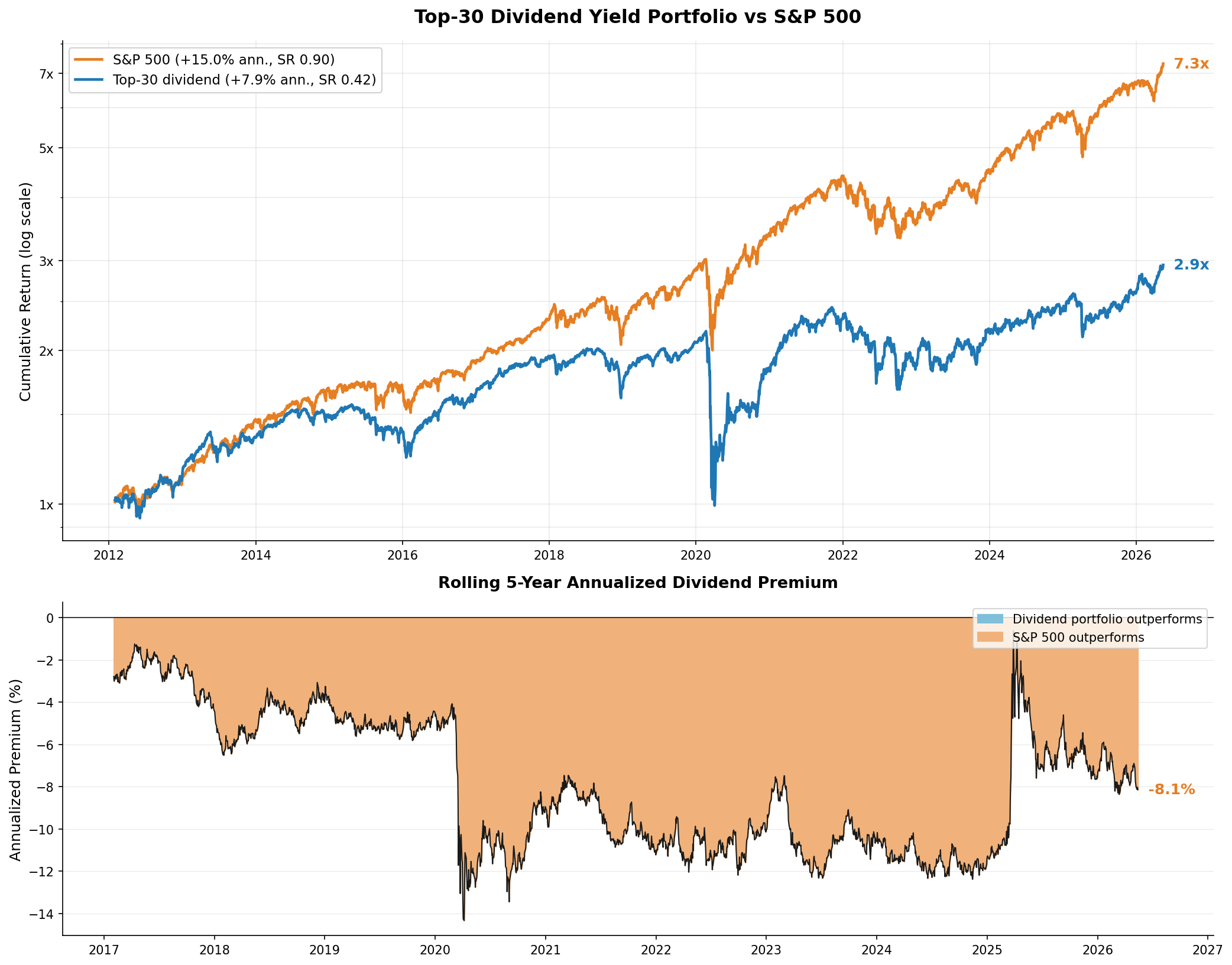
Full sample: 7.9% annualised vs 15.0% for the S&P 500, Sharpe 0.42 vs 0.90. A dollar compounded to $2.9 in the dividend portfolio and $7.3 in the index.
The rolling 5-year premium has been negative through almost the entire sample, currently at −8.1%.
There are several configurations for dividend portfolios, and this portfolio is the simplest one you can go with. But in this setting, it does not pay off to follow it.
This does not mean a dividend tilt cannot work. It means that, historically, a pure yield ranking with no other filter has lost to the S&P 500 over this window. Filtering on payout sustainability, free cash flow coverage, or quality could be a next step.
Caveats
Yield-trap risk beyond the MC floor. A 25% yield on a $1 billion stock is still usually a price-collapse signal. The $500m floor drops the worst, but the portfolio still picks up some of these. A payout-ratio screen would help; this version does not have one.
Sector concentration. Some months the top 30 by yield are concentrated in a single sector (REITs in 2020, traditional energy in 2022). Equal-weight across the 30 names does not stop the sector tilt.
Effective start ~2012. TR.DividendYield is sparsely populated in the LSEG pull before 2012. The MIN_HOLDINGS = 25 filter skips the warm-up months, so the displayed strategy effectively starts in 2012 rather than 2011.
Market impact beyond the quoted spread. The cost model charges the half-spread and a commission. Real execution shows slippage past top-of-book, and Hagströmer and Hübbert (2026) show conventional trade-quote matching algorithms (Lee–Ready and variants) overstate effective spreads by roughly 8–18% — so the half-spread itself is a noisy proxy. Another 30–80 bps a year of total drag is plausible on a $500m-floor strategy.
Data source
US equity total returns, dividend yields, market caps, and bid-ask quotes pulled from LSEG Workspace (licensed). The download pipeline is in an earlier post, with the universe set to all US common stocks on NYSE and Nasdaq.
Disclaimer: simplified, hypothetical backtest with approximate trading costs for discussion purposes only. Not investment advice. Past performance does not predict future returns.