Do stocks still drift after earnings announcements?
It is currently earnings season, and companies are releasing their earnings announcements. There is a famous pattern called post-earnings-announcement drift (PEAD), which Ball and Brown (1968) showed. After a company has made its earnings announcement, its stock return continues to move in the same direction as the reaction to the announcement. The question I want to ask is whether that still holds today, going back at least five years.
The data
I gather daily data from the London Stock Exchange Group (LSEG) on about 10,000 US stocks from January 2000 to February 2026, and I leave out any stock priced below $5. That gives me 285,170 announcements.
Unfortunately, the data do not include announcement dates, so I infer them from changes in earnings before interest and taxes (EBIT). The change in EBIT appears in the data before the earnings announcement, and I do not know why that is the case. So the announcement is on the day after the change, which I call day 0.
Some companies announce earnings after the close, so the reaction comes on day 1. So I compute the stock return on days 0 and 1, and I subtract the return of stocks of the same size to get an excess return. I also include day -1, because some companies report a day before the date I infer. As in the research, the stocks of the same size include those that report on the same days.
Within each quarter, I rank all announcements by reaction and split them into 10 equal-sized groups. Group 1 is the group with the weakest reactions, those that fell the most, and group 10 is the one with the strongest, those that increased the most. The reason why I use the cutoffs of the prior quarter is that, when companies are reporting, I do not know exactly what the cutoffs will be until all stocks have reported, while the cutoffs of the prior quarter are known.
Drift is how much the stock return changes relative to stocks of the same size after the reaction, and I measure it from the close of day 1 because some companies report after the close on day 0, so the reaction comes on day 1. The point of view is that of an investor who looks at the final reaction, which cannot be seen until just before the close on day 1. The returns I compute are buy-and-hold: I buy each stock and hold it until day 20, four weeks after the announcement.
\[ \begin{aligned} \text{reaction}_i &= \prod_{d=-1}^{1} (1 + r_{i,d}) - \prod_{d=-1}^{1} (1 + b_{i,d})\\[4pt] \text{drift}_i(k) &= \prod_{d=2}^{k} (1 + r_{i,d}) - \prod_{d=2}^{k} (1 + b_{i,d})\\[4pt] \text{gap}(k) &= \text{drift}(k) \text{ of group 10}\\ & \quad - \text{drift}(k) \text{ of group 1}\\[4pt] \text{with: } & r_{i,d} = \text{the return of stock } i \text{ on day } d\\ & b_{i,d} = \text{the return of stocks of the}\\ & \quad \text{same size as stock } i \text{ on day } d\\ & k = \text{the day the drift is measured} \end{aligned} \]
Companies report during similar periods, in clusters, and the same market moves can hit them, so they are not independent of each other; that is why I average each quarter and compute a t-value adjusted for that, using Newey-West standard errors.
Results
| Return minus same-size stocks |
|---|
Faded lines: 2000 to 2025
From 2000 to 2025, the stocks with the strongest reaction rise 0.65 percentage points more than stocks with a similar market cap by day 20, while those with the weakest reaction fall 0.08 points more. The gap between the strongest and weakest group is 0.73 points with a t-value of 3.59, which is statistically different from zero. The fall of the weakest group on its own is not statistically significant.
But from 2020, the gap is 0.32 points, mainly because the weakest group rises by 0.18 points. Instead of falling in the four weeks after the announcement, those stocks are rising, so the gap between the strongest and the weakest group is smaller, and it comes with a t-value of 0.59, which suggests that it is not statistically different from zero. The drop of 0.54 points from before 2020 is not statistically significant either.
| Period | Gap by day 20 (percentage points) | t-value |
|---|---|---|
| 2000 to 2025 | 0.73 | 3.59 |
| 2000 to 2019 | 0.86 | 4.23 |
| 2020 to 2025 | 0.32 | 0.59 |
I also compute the alpha of a strategy going long in the strongest group and short in the weakest, which is the return that the market, size, value, and momentum factors do not explain, and the alpha is narrowing down, from 0.59% a month before 2020 to 0.10% a month from 2020.
Limitations
I need to infer the announcement dates. Returns are systematically larger on these dates, which is strong confirmation. For a sample of 11 companies, I compared the dates with their filings at the Securities and Exchange Commission (SEC). For 10 of them, the earnings release falls within days -1 to 1.
I do not include any trading costs.
I go back six years, to 2020, which gives fewer observations, but a more updated view. Starting the recent period in any year from 2010 to 2018 gives the same result, with a gap that is never statistically different from zero.
Conclusion
So the conclusion is that yes, there is a drift from 2000 to 2025. In the recent period, the last six years, there is still a gap, but it is not statistically different from zero. So it is possible that, although there has been a drift, it still exists but with a much smaller magnitude, if not zero. Trading on PEAD may not be as profitable as it once was.
Appendix: the code
from pathlib import Path
import json
import cv2
import numpy as np
import pandas as pd
import matplotlib.pyplot as plt
import statsmodels.api as sm
from matplotlib.lines import Line2D

FOLDER = Path.cwd()
STOCKS_FILE = FOLDER / "Data" / "US_stocks.csv"
FRENCH = "https://mba.tuck.dartmouth.edu/pages/faculty/ken.french/ftp/"
FACTORS_URL = FRENCH + "F-F_Research_Data_Factors_CSV.zip"
MOMENTUM_URL = FRENCH + "F-F_Momentum_Factor_CSV.zip"
MIN_PRICE = 5
MIN_GAP = 40
CHART_DAYS = 20
LAST_DAY = 61
RECENT_START = 2020
LEVELS = [i / 10 for i in range(1, 10)]def window(table, day0, columns, first, last):
days = day0[:, None] + np.arange(first, last + 1)
return table[days, columns[:, None]]
def compounded(returns):
return 100 * (np.cumprod(1 + returns, axis=1) - 1)
def decile_of(values, cutoffs):
return cutoffs.lt(values, axis=0).sum(axis=1)
def mean_and_t(series, lags):
model = sm.OLS(series.to_numpy(), np.ones(len(series)))
fit = model.fit(cov_type="HAC", cov_kwds={"maxlags": lags})
return fit.params[0], fit.tvalues[0]
def monthly_rows(table):
table = table[table.index.astype(str).str.strip().str.len() == 6].astype(float)
table.index = pd.to_datetime(table.index.astype(str).str.strip(), format="%Y%m")
table.index = table.index.to_period("M")
return table
drift_test = compounded(np.full((1, 19), 0.01))[0, -1] - compounded(np.full((1, 19), 0.005))[0, -1]
window_test = window(np.arange(12).reshape(6, 2), np.array([2]), np.array([1]), -1, 1)
nine_cutoffs = pd.DataFrame([list(range(1, 10))] * 3, columns=LEVELS)
cutoff_test = decile_of(pd.Series([0.5, 5.0, 9.5]), nine_cutoffs)
print("Do the functions give the hand-computed answers?",
np.isclose(drift_test, 100 * (1.01**19 - 1.005**19)) and window_test.tolist() == [[3, 5, 7]]
and cutoff_test.tolist() == [0, 4, 9])Do the functions give the hand-computed answers? Truecolumns = ["Instrument", "Date", "Daily Total Return", "Company Market Cap", "Bid Price",
"Ask Price", "EBIT"]
text_columns = {"Instrument": "category", "Date": "category"}
stocks = pd.read_csv(STOCKS_FILE, usecols=columns, dtype=text_columns)
stocks["Date"] = pd.to_datetime(stocks["Date"], format="%Y-%m-%d").astype("datetime64[ns]")
rows_per_date = stocks["Date"].value_counts().sort_index()
usual_rows = rows_per_date.rolling(21, center=True, min_periods=1).median()
trading_days = rows_per_date.index[rows_per_date >= 0.5 * usual_rows]
stocks = stocks[stocks["Date"].isin(trading_days)].sort_values(["Instrument", "Date"])
day_number = pd.Series(range(len(trading_days)), index=trading_days)
stocks["day"] = stocks["Date"].map(day_number).to_numpy()
stocks["stock"] = stocks["Instrument"].cat.codes.to_numpy()
stocks["price"] = (stocks["Bid Price"] + stocks["Ask Price"]) / 2
cap_change = 100 * stocks.groupby("stock")["Company Market Cap"].pct_change(fill_method=None)
move = stocks["Daily Total Return"]
confirmed = (np.sign(cap_change) == np.sign(move)) & (cap_change.abs() >= move.abs() / 2)
stocks.loc[(move.abs() > 50) & ~confirmed, "Daily Total Return"] = np.nan
n_days, n_stocks = len(trading_days), len(stocks["Instrument"].cat.categories)
day, stock = stocks["day"].to_numpy(), stocks["stock"].to_numpy()
returns = np.full((n_days, n_stocks), np.nan)
returns[day, stock] = stocks["Daily Total Return"].to_numpy() / 100
caps_before = np.full((n_days, n_stocks), np.nan)
has_next = day + 1 < n_days
caps_before[day[has_next] + 1, stock[has_next]] = stocks["Company Market Cap"].to_numpy()[has_next]
print(f"Rows: {len(stocks):,}; stocks: {n_stocks:,}; trading days: {n_days:,}, "
f"{trading_days[0]:%Y-%m-%d} to {trading_days[-1]:%Y-%m-%d}")Rows: 27,421,968; stocks: 10,078; trading days: 6,574, 2000-01-03 to 2026-02-27month_list = pd.period_range(trading_days[0], trading_days[-1], freq="M")
month_number = pd.Series(range(len(month_list)), index=month_list)
month_of_day = trading_days.to_period("M").map(month_number).to_numpy()
stocks["month"] = month_of_day[stocks["day"].to_numpy()]
month_ends = stocks.drop_duplicates(["stock", "month"], keep="last")
month_ends = month_ends.dropna(subset=["Company Market Cap"])
is_nyse = month_ends["Instrument"].astype(str).str.contains(r"\.N(?:\^|$)")
cutoffs = month_ends[is_nyse].groupby("month")["Company Market Cap"].quantile(LEVELS).unstack()
month_ends = month_ends.merge(cutoffs, left_on="month", right_index=True)
month_ends["decile"] = decile_of(month_ends["Company Market Cap"], month_ends[LEVELS])
month_ends = month_ends[month_ends["month"] + 1 < len(month_list)]
next_month, columns_next = month_ends["month"].to_numpy() + 1, month_ends["stock"].to_numpy()
size_decile = np.full((len(month_list), n_stocks), -1, dtype=np.int8)
size_decile[next_month, columns_next] = month_ends["decile"].to_numpy()
priced = np.zeros((len(month_list), n_stocks), dtype=bool)
priced[next_month, columns_next] = (month_ends["price"] >= MIN_PRICE).to_numpy()
decile_by_day = size_decile[month_of_day]
member = priced[month_of_day] & ~np.isnan(returns) & ~np.isnan(caps_before)
weighted = caps_before * returns
benchmark = np.full((n_days, 10), np.nan)
for decile in range(10):
in_decile = member & (decile_by_day == decile)
total = np.where(in_decile, caps_before, 0).sum(axis=1)
benchmark[:, decile] = np.divide(np.where(in_decile, weighted, 0).sum(axis=1), total,
out=np.full(n_days, np.nan), where=total > 0)report_columns = ["stock", "day", "EBIT", "Company Market Cap", "price"]
reports = stocks.loc[stocks["EBIT"].notna(), report_columns]
previous = reports.groupby("stock")["EBIT"].shift(1)
changes = reports[previous.notna() & (reports["EBIT"] != previous)]
keep, last_kept = [], {}
for stock_id, change_day in zip(changes["stock"], changes["day"]):
keep.append(change_day - last_kept.get(stock_id, -MIN_GAP) >= MIN_GAP)
if keep[-1]:
last_kept[stock_id] = change_day
events = changes[keep].rename(columns={"Company Market Cap": "cap"})
events["day0"] = events["day"] + 1
events["next_day0"] = events.groupby("stock")["day0"].shift(-1)
inside = events["day0"] + LAST_DAY < n_days
priced_and_valued = (events["price"] >= MIN_PRICE) & events["cap"].notna()
events = events[inside & priced_and_valued]
events["decile"] = size_decile[month_of_day[events["day0"].to_numpy()], events["stock"].to_numpy()]
events = events[events["decile"] >= 0].reset_index(drop=True)
day0 = events["day0"].to_numpy()
stock_returns = window(returns, day0, events["stock"].to_numpy(), -1, LAST_DAY)
benchmark_returns = window(benchmark, day0, events["decile"].to_numpy(), -1, LAST_DAY)
usable = ~np.isnan(stock_returns[:, :3]).any(axis=1) & ~np.isnan(benchmark_returns).any(axis=1)
events = events[usable].reset_index(drop=True)
stock_returns, benchmark_returns = stock_returns[usable], benchmark_returns[usable]
stock_returns = np.where(np.isnan(stock_returns), benchmark_returns, stock_returns)
reaction = compounded(stock_returns[:, :3])[:, -1] - compounded(benchmark_returns[:, :3])[:, -1]
events["reaction"] = reaction
events["quarter"] = trading_days[events["day0"].to_numpy()].to_period("Q")
quarter_cutoffs = events.groupby("quarter")["reaction"].quantile(LEVELS).unstack()
quarter_cutoffs.index = quarter_cutoffs.index + 1
cutoffs_by_event = quarter_cutoffs.reindex(events["quarter"]).reset_index(drop=True)
has_cutoffs = cutoffs_by_event.notna().all(axis=1).to_numpy()
events["group"] = decile_of(events["reaction"], cutoffs_by_event) + 1
events = events[has_cutoffs].reset_index(drop=True)
stock_returns, benchmark_returns = stock_returns[has_cutoffs], benchmark_returns[has_cutoffs]
events["year"] = trading_days[events["day0"].to_numpy()].year
first_year, last_year = int(events["year"].min()), int(events["year"].max())
print(f"Announcements: {len(events):,}, day 0 from {first_year} to {last_year}")
change_day = events["day"].to_numpy()
around = (window(returns, change_day, events["stock"].to_numpy(), -3, 4)
- window(benchmark, change_day, events["decile"].to_numpy(), -3, 4))
day_check = pd.Series(100 * np.nanmean(np.abs(around), axis=0), index=range(-3, 5))
print("Mean absolute excess return, %, by trading day after the EBIT change:")
print(day_check.round(2).to_string())Announcements: 285,170, day 0 from 2000 to 2025
Mean absolute excess return, %, by trading day after the EBIT change:
-3 1.53
-2 1.54
-1 1.55
0 1.82
1 3.14
2 3.45
3 1.93
4 1.72drift = compounded(stock_returns[:, 3:]) - compounded(benchmark_returns[:, 3:])
drift = pd.DataFrame(drift, columns=range(2, LAST_DAY + 1))
chart_days = list(range(2, CHART_DAYS + 1))
quarterly = drift[chart_days].groupby([events["quarter"], events["group"]]).mean()
by_quarter = quarterly[CHART_DAYS].unstack()
gap = by_quarter[10] - by_quarter[1]
years = by_quarter.index.year
periods = {f"{first_year} to {last_year}": years >= first_year,
f"{first_year} to {RECENT_START - 1}": years < RECENT_START,
f"{RECENT_START} to {last_year}": years >= RECENT_START}
groups = {"strongest group": by_quarter[10], "weakest group": by_quarter[1], "gap": gap}
rows = []
for period, in_period in periods.items():
for group, series in groups.items():
mean, t = mean_and_t(series[in_period], 1)
rows.append({"period": period, "group": group, "drift to day 20, %": mean, "t-value": t})
tests = pd.DataFrame(rows)
print(tests.round(2).to_string(index=False))
from_recent = pd.Series((years >= RECENT_START).astype(float), index=gap.index, name="from recent")
change = sm.OLS(gap, sm.add_constant(from_recent)).fit(cov_type="HAC", cov_kwds={"maxlags": 1})
print(f"\nChange in the gap from {RECENT_START}: {change.params['from recent']:.2f} points, "
f"t-value {change.tvalues['from recent']:.2f}")
start_years = []
for start in range(2010, RECENT_START + 1, 2):
mean, t = mean_and_t(gap[years >= start], 1)
quarters = int((years >= start).sum())
start_years.append({"from": start, "quarters": quarters, "gap": mean, "t-value": t})
print("\nThe gap from other start years:")
print(pd.DataFrame(start_years).round(2).to_string(index=False)) period group drift to day 20, % t-value
2000 to 2025 strongest group 0.65 3.93
2000 to 2025 weakest group -0.08 -0.50
2000 to 2025 gap 0.73 3.59
2000 to 2019 strongest group 0.70 3.75
2000 to 2019 weakest group -0.16 -0.90
2000 to 2019 gap 0.86 4.23
2020 to 2025 strongest group 0.50 1.44
2020 to 2025 weakest group 0.18 0.46
2020 to 2025 gap 0.32 0.59
Change in the gap from 2020: -0.54 points, t-value -0.96
The gap from other start years:
from quarters gap t-value
2010 64 0.45 1.63
2012 56 0.40 1.32
2014 48 0.33 0.98
2016 40 0.24 0.63
2018 32 0.25 0.56
2020 24 0.32 0.59french_factors = pd.read_csv(FACTORS_URL, skiprows=4, index_col=0)
french_momentum = pd.read_csv(MOMENTUM_URL, skiprows=13, index_col=0)
factors = monthly_rows(french_factors)[["Mkt-RF", "SMB", "HML"]]
factors = factors.join(monthly_rows(french_momentum)["Mom"])
side = np.select([events["group"] == 10, events["group"] == 1], ["long", "short"], "")
chosen = np.flatnonzero(side != "")
first_held = events["day0"].to_numpy() + 2
next_start = events["next_day0"].fillna(np.inf).to_numpy()
last_held = np.minimum(events["day0"].to_numpy() + LAST_DAY, next_start - 1).astype(int)
holdings = pd.DataFrame({"event": np.repeat(chosen, last_held[chosen] - first_held[chosen] + 1)})
holdings["side"] = side[holdings["event"]]
holdings["day"] = first_held[holdings["event"]] + holdings.groupby("event").cumcount().to_numpy()
event_day0 = events["day0"].to_numpy()[holdings["event"]]
column = holdings["day"].to_numpy() - event_day0 + 1
holdings["return"] = stock_returns[holdings["event"].to_numpy(), column]
daily = holdings.groupby(["day", "side"])["return"].agg(["mean", "size"]).reset_index()
daily = daily[daily["size"] >= 10].pivot(index="day", columns="side", values="mean").dropna()
month = trading_days[daily.index.to_numpy()].to_period("M")
monthly = (1 + daily[["long", "short"]]).groupby(month).prod() - 1
months = factors.reindex(monthly.index)
months["long-short"] = 100 * (monthly["long"] - monthly["short"])
months = months.dropna()
four_factors = ["Mkt-RF", "SMB", "HML", "Mom"]
alphas = {}
for period, in_period in [(f"before {RECENT_START}", months.index.year < RECENT_START),
(f"from {RECENT_START}", months.index.year >= RECENT_START)]:
sample = months[in_period]
model = sm.OLS(sample["long-short"], sm.add_constant(sample[four_factors]))
fit = model.fit(cov_type="HAC", cov_kwds={"maxlags": 3})
alphas[period] = {"months": len(sample), "alpha": fit.params["const"],
"t-value": fit.tvalues["const"]}
print("Four-factor alpha of the long-short strategy, % a month:")
print(pd.DataFrame(alphas).T.round(2).to_string())Four-factor alpha of the long-short strategy, % a month:
months alpha t-value
before 2020 237.0 0.59 4.11
from 2020 74.0 0.10 0.31quarter_rows = quarterly.reset_index()
starts = {f"{first_year} to {last_year}": first_year,
f"{RECENT_START} to {last_year}": RECENT_START}
curves = {}
for title, start in starts.items():
in_period = quarter_rows["quarter"].dt.year >= start
period_curves = quarter_rows[in_period].groupby("group")[chart_days].mean()
period_curves.insert(0, 1, 0.0)
curves[title] = period_curves
TEAL, ORANGE, GREY = "#17868A", "#D2822B", "#888888"
BG, INK, GRID = "#FCEFE3", "#1f1f1f", "#EADCCC"
SPINE, AXIS_TEXT, TICK_TEXT = "#D5C6B4", "#4a4a4a", "#7a7168"
LINES = {10: (TEAL, "Strongest reactions"), 1: (ORANGE, "Weakest reactions")}
def style_chart(figure, axis):
figure.patch.set_facecolor(BG)
axis.set_facecolor(BG)
axis.grid(True, axis="y", color=GRID, lw=1.0)
axis.set_axisbelow(True)
for side_name in ("top", "right"):
axis.spines[side_name].set_visible(False)
for side_name in ("left", "bottom"):
axis.spines[side_name].set_color(SPINE)
axis.tick_params(axis="both", length=0, pad=6, labelsize=12.5, labelcolor=TICK_TEXT)
axis.xaxis.label.set_color(AXIS_TEXT)
axis.yaxis.label.set_color(AXIS_TEXT)
axis.title.set_color(INK)
fig, axes = plt.subplots(1, 2, figsize=(12, 8), sharey=True)
for ax, title in zip(axes, curves):
for group, (color, label) in LINES.items():
line = curves[title].loc[group]
ax.plot(line.index, line, color=color, lw=3.2, marker="o", ms=5, label=label)
ax.axhline(0, color=GREY, lw=1.2, ls="--")
ax.set_xticks([1, 5, 10, 15, 20])
ax.set_title(title, fontsize=15)
ax.set_xlabel("Trading days after the announcement", fontsize=14)
style_chart(fig, ax)
axes[0].set_ylabel("Return minus same-size stocks (%)", fontsize=14)
handles, labels = axes[0].get_legend_handles_labels()
legend = fig.legend(handles, labels, loc="upper center", ncol=2, frameon=False, fontsize=13)
for text, handle in zip(legend.get_texts(), legend.legend_handles):
text.set_color(handle.get_color())
fig.tight_layout(rect=(0, 0, 1, 0.94))
fig.savefig(FOLDER / "earnings_drift.png", dpi=200, facecolor=BG, bbox_inches="tight")
plt.show()
numbers = {"announcements": len(events), "first_year": first_year, "last_year": last_year,
"curves": {title: {str(group): c.loc[group].tolist() for group in LINES}
for title, c in curves.items()},
"tests": tests.to_dict("records"),
"change": [change.params["from recent"], change.tvalues["from recent"]],
"start_years": start_years, "alphas": alphas, "day_check": day_check.to_dict()}
(FOLDER / "earnings_drift_numbers.json").write_text(json.dumps(numbers, indent=1), encoding="utf-8")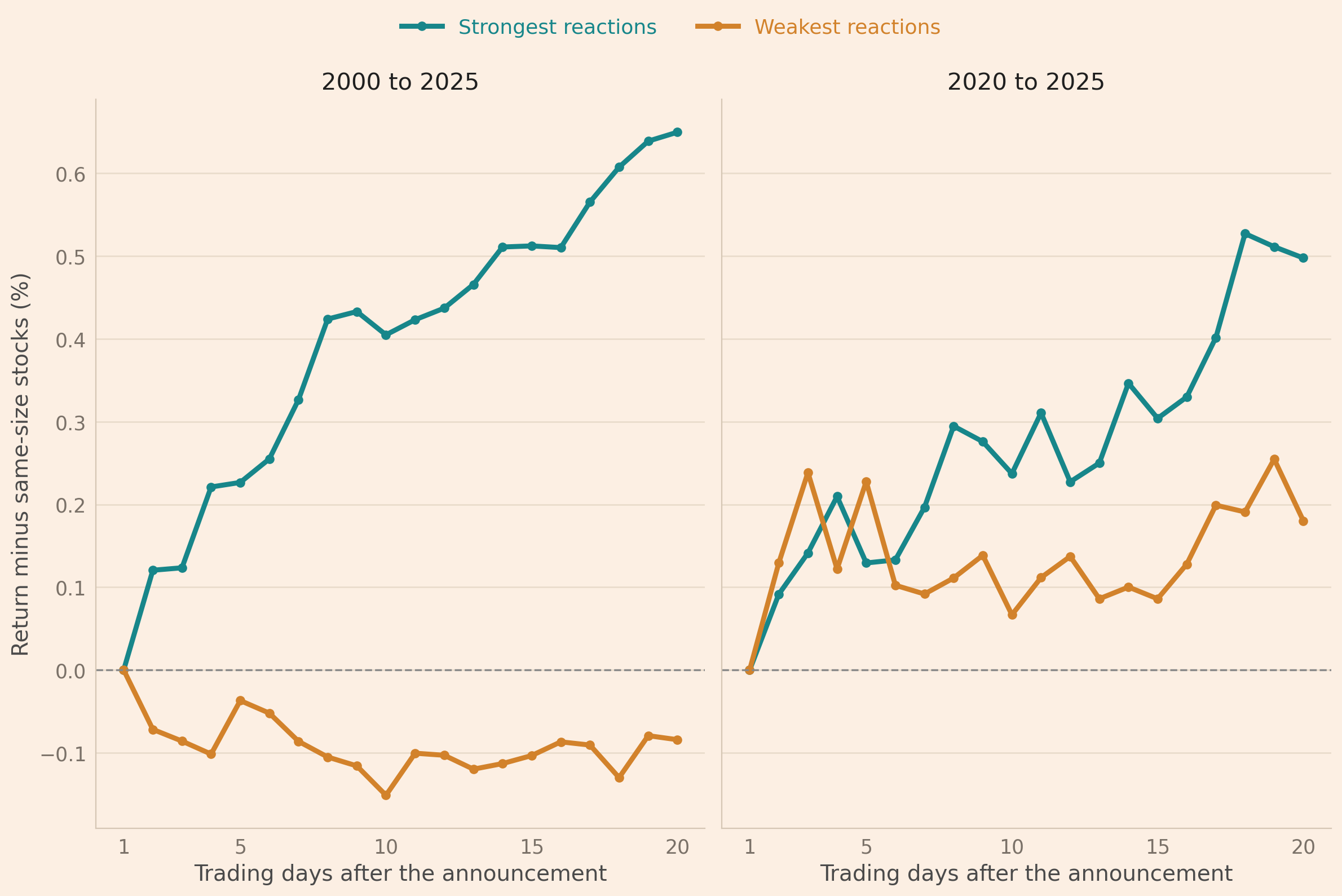
VIDEO_W, VIDEO_H, VIDEO_DPI, FPS = 1440, 960, 120, 60
DRAW, HOLD, FADE, END, FADED = 180, 90, 45, 300, 0.25
full_title, recent_title = list(curves)
values = np.concatenate([curves[title].loc[group].to_numpy()
                         for title in curves for group in LINES])
y_limits = (values.min() - 0.1, values.max() + 0.1)


def smoothstep(u):
    u = min(max(u, 0.0), 1.0)
    return u * u * (3 - 2 * u)


def partial_line(line, progress):
    whole = int(np.floor(progress))
    days, shown = list(range(1, whole + 1)), list(line[:whole])
    if progress > whole:
        days.append(progress)
        shown.append(np.interp(progress, range(1, CHART_DAYS + 1), line))
    return np.array(days), np.array(shown)


video_figure = plt.figure(figsize=(VIDEO_W / VIDEO_DPI, VIDEO_H / VIDEO_DPI), dpi=VIDEO_DPI)


def frame(drawn, full_alpha, badge):
    video_figure.clf()
    axis = video_figure.add_axes([0.088, 0.115, 0.875, 0.73])
    for title, progress in drawn.items():
        alpha = full_alpha if title == full_title else 1.0
        for group, (color, label) in LINES.items():
            days, shown = partial_line(curves[title].loc[group].to_numpy(), progress)
            axis.plot(days, shown, color=color, lw=3.2, alpha=alpha, solid_capstyle="round")
            whole_day = days == np.floor(days)
            axis.plot(days[whole_day], shown[whole_day], "o", ms=6, color=color, alpha=alpha)
    axis.axhline(0, color=GREY, lw=1.2, ls="--")
    axis.set_xlim(0.5, CHART_DAYS + 0.5)
    axis.set_ylim(*y_limits)
    axis.set_xticks([1, 5, 10, 15, 20])
    axis.set_xlabel("Trading days after the announcement", fontsize=14, labelpad=9)
    axis.set_ylabel("Return minus same-size stocks (%)", fontsize=14, labelpad=9)
    style_chart(video_figure, axis)
    handles = [Line2D([0], [0], color=color, lw=3.2, label=label)
               for color, label in LINES.values()]
    if recent_title in drawn:
        handles.append(Line2D([0], [0], color=GREY, lw=3.2, label=f"Faded lines: {full_title}"))
    legend = video_figure.legend(handles=handles, loc="upper left", bbox_to_anchor=(0.08, 0.99),
                                 frameon=False, fontsize=15)
    for text, handle in zip(legend.get_texts(), handles):
        text.set_color(handle.get_color())
    video_figure.text(0.966, 0.93, badge, ha="right", va="center", fontsize=25, color=INK)
    video_figure.canvas.draw()
    return cv2.cvtColor(np.asarray(video_figure.canvas.buffer_rgba()), cv2.COLOR_RGBA2BGR)


codec = cv2.VideoWriter_fourcc("a", "v", "c", "1")
writer = cv2.VideoWriter(str(FOLDER / "earnings_drift.mp4"), codec, FPS, (VIDEO_W, VIDEO_H))
assert writer.isOpened(), "OpenCV could not open the video writer"
for n in range(DRAW):
    progress = 1 + (CHART_DAYS - 1) * smoothstep((n + 1) / DRAW)
    writer.write(frame({full_title: progress}, 1.0, full_title))
still = frame({full_title: CHART_DAYS}, 1.0, full_title)
for _ in range(HOLD):
    writer.write(still)
for n in range(FADE):
    alpha = 1 - (1 - FADED) * smoothstep((n + 1) / FADE)
    writer.write(frame({full_title: CHART_DAYS}, alpha, recent_title))
for n in range(DRAW):
    progress = 1 + (CHART_DAYS - 1) * smoothstep((n + 1) / DRAW)
    writer.write(frame({full_title: CHART_DAYS, recent_title: progress}, FADED, recent_title))
last = frame({full_title: CHART_DAYS, recent_title: CHART_DAYS}, FADED, recent_title)
for _ in range(END):
    writer.write(last)
writer.release()
plt.close(video_figure)
print(f"Saved earnings_drift.mp4, {(2 * DRAW + HOLD + FADE + END) / FPS:.1f} seconds")
Saved earnings_drift.mp4, 13.2 secondsRead next
- Who wins in size and momentum? If I sort stocks by size and momentum, who wins when I compare returns in excess of the market?
- Trading costs more than halved Swedish momentum’s ending value From 2001 to 2025, trading costs cut one krona’s growth in Swedish momentum from 358 kronor to 156, still ahead of the market’s 55.
Disclaimer: historical returns before trading costs. Not investment advice.
Data and sources: London Stock Exchange Group (LSEG), daily US stock data, January 2000 to February 2026 (licensed, not shared). Kenneth R. French, Data Library, Fama/French 3 Factors and Momentum Factor. U.S. Securities and Exchange Commission, EDGAR filings (Form 8-K, item 2.02). Ray Ball and Philip Brown, “An empirical evaluation of accounting income numbers”, Journal of Accounting Research (1968). I publish only results computed from the data.