Trading costs more than halved Swedish momentum’s ending value
A backtest that ignores trading costs overstates what a strategy earns. A momentum strategy on Swedish stocks, which buys the stocks that rose most over the past year, beat the market by a wide margin before costs, and the costs of real trading more than halved its ending value. Jegadeesh and Titman (1993) find that stocks that rose over the past year tend to keep rising over the next few months. I test whether that held on Swedish stocks from 2001 to 2025, and what it cost to trade.
To separate the gross return from the costs, I built three versions of the momentum portfolio. One ignores all costs. One subtracts the trading commission. One also subtracts the bid-ask spread, the gap between the price to buy and the price to sell.
The gross result was large. One krona in the momentum winners grew to 358 kronor before any costs. The same krona in the market index, an equal-weight index of all the Swedish stocks in the test, grew to 55. So, one krona in the winners was worth 6.5 times the market index value before costs.
Then I add the costs of real trading, one layer at a time. A flat commission reduced the ending value from 358 to 321 kronor. The bid-ask spread reduced it further, from 321 to 156. After both layers, one krona still grew to 156 against 55 for the market, so momentum ended above the market index even though costs more than halved the ending value.
The strategy
- Universe: Swedish common stocks, active and delisted, 2001 to 2025, with a market cap (share price times number of shares) above 500 million Swedish kronor (MSEK).
- Signal: 12-2 momentum, the past twelve months of return with the most recent month skipped.
- Portfolio: the top decile by that signal, the tenth of stocks with the highest signal, held in equal weights that are reset each month.
- Costs: a 0.069% commission per trade, then each traded stock’s bid-ask half-spread.
- Benchmark: an equal-weight index of the same eligible stocks.
I skip the most recent month because one-month returns tend to reverse, so including it adds noise to the signal.
Starting point
The backtest runs off one price file of daily total returns, market caps, and bid-ask quotes for the Swedish market. Building it is a separate job that depends on the data vendor. I pull from LSEG Workspace. Because the data is licensed, I cannot share the raw file, and I show the code without running it here.
The printed ending values and the figure come from my run of the full script.
Step 1. The 12-2 momentum signal
Each stock gets one signal a month: its cumulative return over the past year, ending two months back. I work in log space so the twelve monthly returns add up, then convert back.
def twelve_month_sum(log_returns):
    """The sum of the twelve monthly log returns ending at each month."""
    # min_periods=12 leaves the result missing until a stock has a full year behind it,
    # so eleven observed months never pass as a year.
    return log_returns.rolling(12, min_periods=12).sum()


# Log returns add up across months, so a year is the sum of twelve rows rather than a
# product of twelve factors. log1p(r) is log(1 + r).
monthly["log1r"] = np.log1p(monthly["monthly_ret"])

# transform() runs the function inside each stock's own rows and hands the results back in
# the original row order. A rolling window over the whole column would run from the end of
# one stock straight into the start of the next.
twelve_month_log = monthly.groupby("Instrument")["log1r"].transform(twelve_month_sum)

# expm1 undoes log1p, so the summed log returns come back as one ordinary return.
monthly["cum_12m"] = np.expm1(twelve_month_log)

# Lag by one month so the signal at month t stops at the end of month t-2.
monthly["mom_signal"] = monthly.groupby("Instrument")["cum_12m"].shift(1)
The lag makes the signal “12-2”. The shift(1) moves each stock’s own past value forward so the signal that ranks stocks at the start of a month uses only returns that had already happened. Lesson 20 covers the one-month shift.
Step 2. Pick the top decile each month
I rank the eligible stocks each month and keep the highest tenth. The benchmark is the equal-weight return of every eligible stock that same month.
# rank(pct=True) turns each month's signals into shares between 0 and 1, so one cut-off
# means the same thing in a month with 200 stocks and in a month with 400.
monthly["mom_rank"] = monthly.groupby("YM")["mom_signal"].rank(pct=True)

# A boolean mask, one True or False per row. 0.9 is the start of the highest tenth.
in_top_decile = monthly["mom_rank"] >= 0.9
winners = monthly[in_top_decile]

# The benchmark holds every eligible stock in equal weight, so its return for a month is
# the plain average of that month's returns.
market = monthly.groupby("YM")["monthly_ret"].mean()
Step 3. Layer the costs
I walk month by month and compare the winners this month with the winners last month. A stock that stays in the portfolio pays nothing. A stock that enters or leaves pays the commission and half its bid-ask spread. I weight the spread cost by how much of the portfolio trades.
COMMISSION = 0.00069                          # 0.069% per trade

for ym in months:
    # A set holds each name once, and subtracting one set from another leaves the names
    # in the first and not the second. Those two differences are the month's trades.
    held = set(winners_this_month)
    entering = held - held_last_month          # stocks bought this month
    exiting = held_last_month - held           # stocks sold this month

    # Half the bid-ask spread is what one trade gives up against the midpoint, and only
    # the traded part of the portfolio pays it, so each side pays the share of the portfolio it
    # moves.
    cost_of_buying = weight_bought * half_spread(entering)
    cost_of_selling = weight_sold * half_spread(exiting)
    spread_cost = cost_of_buying + cost_of_selling

    # Every buy and every sell pays the flat rate. Dividing the number of trades by the
    # number of holdings turns a rate per trade into a cost on the whole portfolio.
    comm_cost = (len(entering) + len(exiting)) / n_held * COMMISSION

    ret_no_cost = gross_ret                    # raw equal-weight return of the winners
    ret_comm = gross_ret - comm_cost           # after commission
    ret_all = gross_ret - comm_cost - spread_cost   # after commission and spread

    held_last_month = held                     # kept for the next pass of the loop
Turnover is the share of the portfolio bought or sold in a month. The commission and the spread are charged on the same turnover, so they differ only in the rate: a flat 0.069% for the commission against each stock’s own half-spread. Lesson 31 covers how I measure and charge turnover.
Step 4. Compare to the market
I compound one krona through each of the four return series and read off the ending value.
# Each entry pairs the label to print with the column of monthly returns to compound.
series_to_compound = [("No costs", "ret_no_cost"),
                      ("After commission", "ret_comm"),
                      ("After commission + spread", "ret_all"),
                      ("Market index", "market_ret")]

for label, column in series_to_compound:
    monthly_growth = 1 + port[column]          # one krona is worth 1 + r after a month
    # cumprod multiplies each month onto the months before it, so the series holds what
    # one krona is worth at every point. iloc[-1] reads the last row, the end of the run.
    krona_path = monthly_growth.cumprod()
    ending_value = krona_path.iloc[-1]
    print(f"{label:<28} {ending_value:>3.0f}")
No costs 358
After commission 321
After commission + spread 156
Market index 55One krona in the winners grew to 358 kronor with no costs, 321 after the commission and 156 after the spread, against 55 for the market index. So the commission removed 37 kronor of the ending value and the spread 165.
Results
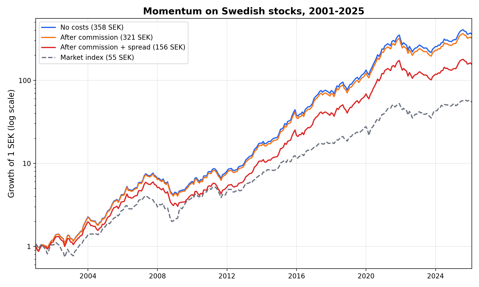
The three momentum lines are close together until the mid-2010s, then the after commission plus spread line is increasingly below the other two. All three stay above the market index for the whole sample. The no costs line and the after commission plus spread line both increase over the sample. The vertical distance between those two lines at the end of the sample is what the trading costs took.
Limitations
The spread cost comes from turnover. A monthly top-decile rebalance replaces much of the portfolio each month and pays the spread on each replacement. The reduction from 358 to 156 kronor is mostly this repeated spread. I do not test a slower rebalance.
The spread is a median estimate. I use each stock’s median bid-ask spread, the middle value of its quoted spreads, and charge half of it. Real fills are worse than the quoted midpoint in small and thinly traded stocks, which the momentum portfolio holds many of, so the true spread cost is higher than the number here.
No market impact. I model the spread and the commission and stop there, following Novy-Marx and Velikov (2016). A large order pushes the price as it fills, and that impact would lower the after commission plus spread line further.
One specification. Top decile, monthly rebalance, equal weight, a 500 MSEK floor, and monthly returns with their extreme values capped, called winsorised, are all choices. I do not report results for other choices, and I do not calculate a confidence interval, a range that likely contains the true value.
Conclusion
Momentum in Sweden ended 303 kronor above the market index before costs, and trading costs removed 202 kronor of that difference, 37 through the commission and 165 through the spread, leaving the winners well ahead of the market index. Other mistakes can also make a backtest overstate what a strategy earns, such as tuning it to the noise in past data or leaving out delisted stocks, and this post measures the trading costs only. The takeaway is that momentum ended above the market index after realistic trading costs in this sample, and the bid-ask spread removed far more of the gross return than the commission did.
Read next
- The Magic Formula worked. Just not lately. Another published edge on US stocks, and how it performed after publication.
- Does your backtested Sharpe ratio show a real edge? One of the other things that inflate a backtest: too few observations behind a Sharpe ratio.
Disclaimer: simplified, hypothetical backtest with approximate trading costs, for discussion purposes only. Not investment advice. Past performance does not guarantee future returns.
Update: an earlier version of this backtest gave different ending values for the three versions of the momentum portfolio. The market index and the conclusion are the same.
Data: Swedish equity daily total returns, market caps, and bid-ask quotes from LSEG Workspace (licensed). I do not reproduce the raw file here.