How to calculate abnormal returns for large stocks without bias
When estimating the abnormal returns of large stocks, for example in an event study, the abnormal returns can be biased by the way they are estimated. A common approach is the market model, which estimates a stock’s beta relative to the market return. For a large stock, the market return and the error term, which captures company-specific news, are not independent. If NVIDIA had an excellent report, for example, it would also move the market. The market model then attributes part of NVIDIA’s price increase to the market rather than to the earnings announcement. As a result, the estimated normal return is too high, and the abnormal return is understated. This bias grows with the stock’s weight in the market used to estimate beta, its beta and the volatility of its company-specific news, so it matters most for large stocks.
I show how much the market model understates or overstates the abnormal returns of a large stock, using simulated data where the true values are known, and how Lally and Swidler’s (2003) proposal removes the bias.
Step 1. Simulating stock returns and earnings announcements
I simulate a stock market where the true abnormal return is known so that I can compare Lally and Swidler’s (2003) proposal with the standard approach.
The market has 500 stocks, similar to the S&P 500, and it trades on every weekday of 2023 and 2024. A stock’s daily return is its beta times the market’s common move plus its company-specific news, which is the stock’s true abnormal return.
I focus on one of the large stocks, S001, which is 7% of the market at the start of 2023. Its true beta is 2, and like the other stocks, it announces earnings four times a year. Its true abnormal returns on the four announcement days in 2024 are +10%, -8%, +14% and -12%.
The simulated data form a panel, because that is the format of a download from a data provider. The columns are the date, the ticker, a flag for an earnings announcement, the total return, the market cap, and the market return, which is the cap-weighted return of all 500 stocks. The last column, the true abnormal return, exists only because the data are simulated.
- Each row is a stock-day.
- The market’s daily common move has a normal distribution with a mean of 0.04% and a standard deviation of 1%.
- Each stock’s beta has a normal distribution with a mean of 1 and a standard deviation of 0.3. I restrict the betas to be at least 0.3 and no more than 2, with S001’s beta set to 2. I then multiply all other stocks’ betas by about 0.9, so that the cap-weighted average beta of the 500 stocks is 1 at the start of 2023. Without that multiplication, it would be 1.1.
- Each stock’s daily company-specific news has a normal distribution with a mean of 0 and its own standard deviation, between 1% and 2.5%. For S001, the standard deviation is 1.5%.
- I assign each stock one random earnings announcement day in each of February, May, August, and November. On an earnings announcement day, a stock’s company-specific news has a standard deviation of 3%. I set S001’s company-specific news on its four announcement days to +9%, -9%, +12%, and -12% in 2023, and to +10%, -8%, +14%, and -12% in 2024.
- I adjust S001’s company-specific news on its 2023 days without an earnings announcement so its average is exactly 0, preventing a nonzero average from affecting the estimation of the normal return.
- The stocks’ market caps at the start of 2023 have a lognormal distribution with a median of $20 billion, with S001 weighted at 7% of the total. The market return weights each stock by its market cap at the previous close.
import numpy as np
import pandas as pd

SEED = 11
N_STOCKS = 500
FACTOR_MEAN = 0.0004
FACTOR_SD = 0.01
EARNINGS_MONTHS = ["2023-02", "2023-05", "2023-08", "2023-11", "2024-02", "2024-05", "2024-08", "2024-11"]
EARNINGS_NEWS_SD = 0.03
LARGE = "S001"
LARGE_WEIGHT = 0.07
LARGE_BETA = 2.0
LARGE_NEWS_SD = 0.015
LARGE_EARNINGS_NEWS = [0.09, -0.09, 0.12, -0.12, 0.10, -0.08, 0.14, -0.12]

rng = np.random.default_rng(SEED)
days = pd.bdate_range("2023-01-01", "2024-12-31")
tickers = [f"S{number:03d}" for number in range(1, N_STOCKS + 1)]

earnings = np.zeros((len(days), N_STOCKS), dtype=bool)
for month in EARNINGS_MONTHS:
    earnings[rng.choice(np.flatnonzero(days.strftime("%Y-%m") == month), N_STOCKS), np.arange(N_STOCKS)] = True
earnings = pd.DataFrame(earnings, index=days, columns=tickers)

start_caps = pd.Series(np.exp(rng.normal(np.log(20e9), 0.8, N_STOCKS)), index=tickers)
start_caps[LARGE] = LARGE_WEIGHT / (1 - LARGE_WEIGHT) * start_caps.drop(LARGE).sum()
start_weights = start_caps / start_caps.sum()
betas = pd.Series(np.clip(rng.normal(1.0, 0.3, N_STOCKS), 0.3, 2.0), index=tickers)
betas[LARGE] = LARGE_BETA
others = betas.index != LARGE
betas[others] *= (1 - LARGE_WEIGHT * LARGE_BETA) / (start_weights[others] * betas[others]).sum()
news_sd = pd.Series(rng.uniform(0.01, 0.025, N_STOCKS), index=tickers)
news_sd[LARGE] = LARGE_NEWS_SD
news = pd.DataFrame(rng.normal(0, 1, (len(days), N_STOCKS)), index=days, columns=tickers) * news_sd
news = news.mask(earnings, pd.DataFrame(rng.normal(0, EARNINGS_NEWS_SD, news.shape), index=days, columns=tickers))
news.loc[earnings[LARGE], LARGE] = LARGE_EARNINGS_NEWS
ordinary_2023 = (days.year == 2023) & ~earnings[LARGE]
news.loc[ordinary_2023, LARGE] -= news.loc[ordinary_2023, LARGE].mean()

market_factor = rng.normal(FACTOR_MEAN, FACTOR_SD, len(days))
returns = news + np.outer(market_factor, betas)
market_caps = (1 + returns).cumprod() * start_caps
caps_before = market_caps.shift(1).fillna(start_caps)
market_return = (caps_before * returns).sum(axis=1) / caps_before.sum(axis=1)

panel = (pd.concat({"earnings_day": earnings.astype(int), "total_return": returns, "market_cap": market_caps,
                    "true_abnormal_return": news}, axis=1)
         .stack(future_stack=True).rename_axis(["date", "ticker"]).reset_index())
panel["market_return"] = panel["date"].map(market_return)
panel = panel[["date", "ticker", "earnings_day", "total_return", "market_cap", "market_return", "true_abnormal_return"]]

print(f"{len(days)} weekdays from {days[0]:%Y-%m-%d} to {days[-1]:%Y-%m-%d}, {N_STOCKS} stocks, "
      f"{len(panel):,} rows")
print(panel.head(3).to_string(index=False))
522 weekdays from 2023-01-02 to 2024-12-31, 500 stocks, 261,000 rows
date ticker earnings_day total_return market_cap market_return true_abnormal_return
2023-01-02 S001 0 0.010617 1.071574e+12 0.007289 -0.005273
2023-01-02 S002 0 0.006374 3.318032e+10 0.007289 -0.003220
2023-01-02 S003 0 -0.013991 3.198866e+10 0.007289 -0.017370Step 2. Estimating the market model with OLS
The market model is the formula below:
\[R_{i,t} = \alpha + \beta R_{m,t} + \varepsilon_{i,t} \tag{1}\]
where \(R_{i,t}\) is the stock return on day \(t\) for stock \(i\), and \(R_{m,t}\) is the market return on day \(t\). \(\beta\) is the stock’s beta, how much the stock’s return changes when the market return increases by 1%. \(\alpha\) is the intercept, the average part of the return that does not depend on the market. \(\varepsilon_{i,t}\) is the error term. The error term is the abnormal return, the part of the return that neither the market nor the intercept can explain, such as company-specific news.
I estimate the beta and the intercept with OLS over 2023, the estimation window:
\[ \begin{gathered} \hat\beta = \frac{\operatorname{Cov}(R_i, R_m)}{\operatorname{Var}(R_m)} \\[8pt] \hat\alpha = \overline{R}_i - \hat\beta\, \overline{R}_m \end{gathered} \tag{2} \]
where the covariance and the variance are over the 2023 trading days, and \(\overline{R}_i\) and \(\overline{R}_m\) are the average stock return and the average market return over the same days.
The normal return, \(\hat\alpha + \hat\beta R_{m,t}\), is the return the market model expects on a given day, and the abnormal return is the rest:
\[AR_{i,t} = R_{i,t} - (\hat\alpha + \hat\beta R_{m,t}) \tag{3}\]
s001 = panel[panel["ticker"] == LARGE].set_index("date")
s001["weight"] = (s001["market_cap"] / panel.groupby("date")["market_cap"].sum()).shift(1).fillna(LARGE_WEIGHT)
s001["others_return"] = (s001["market_return"] - s001["weight"] * s001["total_return"]) / (1 - s001["weight"])


def ols(y, x):
    beta = ((x - x.mean()) * (y - y.mean())).sum() / ((x - x.mean()) ** 2).sum()
    return y.mean() - beta * x.mean(), beta


estimation = s001.loc["2023"]
y, x, z = estimation["total_return"], estimation["market_return"], estimation["others_return"]
alpha_m, beta_m = ols(y, x)
print(f"S001's weight: {s001['weight'].loc['2023'].mean():.2%} on average in 2023, "
      f"{s001['weight'].loc['2024'].mean():.2%} on average in 2024")
print(f"Market model on the market return: alpha {alpha_m:.5f}, beta {beta_m:.3f}")
S001's weight: 7.14% on average in 2023, 7.40% on average in 2024
Market model on the market return: alpha 0.00023, beta 2.211For S001, the market model estimates a beta of 2.21, against the true beta of 2.
Step 3. Why the market model beta is biased for a large stock
OLS gives an unbiased beta only under assumptions about the error term, and the nature of the variables can violate those assumptions. Putting equation (1) into equation (2) gives the estimate \(\hat\beta\) as the true beta \(\beta\), the stock’s response to the market apart from its company-specific news, plus a second part:
\[ \begin{aligned} \hat\beta &= \frac{\operatorname{Cov}(\alpha + \beta R_m + \varepsilon_i,\, R_m)}{\operatorname{Var}(R_m)} \\ &= \frac{\beta\, \operatorname{Var}(R_m) + \operatorname{Cov}(R_m, \varepsilon_i)}{\operatorname{Var}(R_m)} \\ &= \beta + \frac{\operatorname{Cov}(R_m, \varepsilon_i)}{\operatorname{Var}(R_m)} \end{aligned} \tag{4} \]
The estimate is unbiased if the second part averages zero. The market model assumes that the error term averages zero whatever the market return, \(E[\varepsilon_{i,t} \mid R_m] = 0\). The second part then averages zero, and \(E[\hat\beta \mid R_m] = \beta\).
For a large stock, the market return contains part of the company-specific news, because the stock is part of the market:
\[R_{m,t} = w R_{i,t} + (1 - w) R_{n,t} \tag{5}\]
where \(w\) is the stock’s weight in the market, taken as constant, and \(R_{n,t}\) is the return of the other 499 stocks, assumed unrelated to the error term. Putting equation (1) into equation (5) and solving for \(R_{m,t}\) gives:
\[ \begin{aligned} R_{m,t} &= w(\alpha + \beta R_{m,t} + \varepsilon_{i,t}) \\ &\quad + (1 - w) R_{n,t} \\ &= \frac{w(\alpha + \varepsilon_{i,t})}{1 - w\beta} \\ &\quad + \frac{(1 - w) R_{n,t}}{1 - w\beta} \end{aligned} \tag{6} \]
So the company-specific news in the error term moves the market return; the error term does not average to zero whatever the market return, and the estimate is biased.
In equation (6), \(\alpha\) is a constant and \(R_{n,t}\) is unrelated to the error term, so only the term \(w\,\varepsilon_{i,t} / (1 - w\beta)\) moves with the error term, and the covariance between the market return and the error term is:
\[ \begin{aligned} \operatorname{Cov}(R_m, \varepsilon_i) &= \frac{w\, \operatorname{Cov}(\varepsilon_i, \varepsilon_i)}{1 - w\beta} \\ &= \frac{w\, \operatorname{Var}(\varepsilon_i)}{1 - w\beta} \end{aligned} \tag{7} \]
The covariance is positive whenever the stock is part of the market (\(w > 0\)), because the variance of the error term and \(1 - w\beta\) are positive (\(1 - w\beta = 0.86\) for S001). So the second part of equation (4) is positive on average, and the market model’s beta is too high on average. If the error term and the other stocks’ return are normally distributed and independent of each other and across days, the second part averages exactly the covariance in equation (7) divided by the variance of the market return. For a stock outside the market, \(w = 0\), and the second part averages zero.
In the simulation, the true beta is known, so the second part of equation (4) is the market model’s estimate minus the true beta of 2.
second_part = beta_m - LARGE_BETA
true_ar = estimation["true_abnormal_return"]
print(f"Correlation of S001's true abnormal return with the market return {true_ar.corr(x):.2f}, "
      f"with the other stocks' return {true_ar.corr(z):.2f}")
print(f"Market model beta {beta_m:.3f}, true beta {LARGE_BETA:.0f}, second part {second_part:.3f}")
Correlation of S001's true abnormal return with the market return 0.14, with the other stocks' return 0.00
Market model beta 2.211, true beta 2, second part 0.211S001’s true abnormal return has a correlation of 0.14 with the market return and 0.00 with the other stocks’ return. The market model’s estimate is 2.211, so the second part is 0.211.
Step 4. Calculating abnormal returns with both models
Lally and Swidler (2003) estimate the market model on the other stocks’ return in place of the market return, so the normal return takes in none of the company-specific news, as long as that news does not move the other stocks:
\[AR^{n}_{i,t} = R_{i,t} - (\hat\alpha_n + \hat\beta_n R_{n,t}) \tag{8}\]
where \(\hat\alpha_n\) and \(\hat\beta_n\) come from the regression of the stock’s return on \(R_{n,t}\) over 2023.
In the market model, S001’s company-specific news moves the market return in the news’ direction, so the normal return increases on good news and decreases on bad news. The standard abnormal return then understates the size of both good and bad news. On a day when only S001’s company-specific news moves the market, the normal return includes \(w\hat\beta\) of the news: 0.074 × 2.21 = 16.4%, with S001’s average weight in 2024 at 7.4%. Most of it comes from the market return itself. With the true beta of 2, the share would be 0.074 × 2 = 14.8%, and the biased beta adds the other 1.6 percentage points.
alpha_n, beta_n = ols(y, z)
test = s001.loc["2024"].copy()
test["ar_standard"] = test["total_return"] - (alpha_m + beta_m * test["market_return"])
test["ar_lally_swidler"] = test["total_return"] - (alpha_n + beta_n * test["others_return"])
announcements = test[test["earnings_day"] == 1]
print("S001's earnings announcements in 2024 (%)")
print(announcements[["weight", "true_abnormal_return", "ar_standard", "ar_lally_swidler"]].mul(100).round(1)
      .to_string())

true_ar_2024 = test["true_abnormal_return"]
print(f"\nSlope on the true abnormal return over 2024, without an intercept: standard "
      f"{(test['ar_standard'] * true_ar_2024).sum() / (true_ar_2024 ** 2).sum():.2f}, Lally and Swidler "
      f"{(test['ar_lally_swidler'] * true_ar_2024).sum() / (true_ar_2024 ** 2).sum():.2f}")
S001's earnings announcements in 2024 (%)
weight true_abnormal_return ar_standard ar_lally_swidler
date
2024-02-27 7.4 10.0 8.4 9.9
2024-05-21 8.9 -8.0 -6.4 -8.0
2024-08-09 6.1 14.0 12.2 14.2
2024-11-29 7.6 -12.0 -9.9 -12.4
Slope on the true abnormal return over 2024, without an intercept: standard 0.83, Lally and Swidler 1.00On 27 February 2024, S001’s good news was a true abnormal return of +10%, and the standard market model shows +8.4%. On 21 May 2024, its bad news was -8%, and the standard model shows -6.4%. Lally and Swidler’s (2003) model shows +9.9% and -8.0%. Over all trading days of 2024, regressing each model’s abnormal return on the true one, without an intercept, gives a slope of 0.83 for the standard model and 1.00 for Lally and Swidler’s.
Step 5. Cumulative abnormal returns around an earnings announcement
The cumulative abnormal return adds up a stock’s daily abnormal returns from the announcement day:
\[CAR_i(t) = \sum_{s=0}^{t} AR_{i,s} \tag{9}\]
where \(s\) counts the trading days from the announcement, day 0. The lines start at zero on the trading day before S001’s announcement on 27 February 2024.
import matplotlib.pyplot as plt

CHART_DAYS = 5
position = test.index.get_loc(announcements.index[0])
window = test.iloc[position:position + CHART_DAYS + 1]
car = window[["true_abnormal_return", "ar_lally_swidler", "ar_standard"]].cumsum().mul(100)
car = pd.concat([pd.DataFrame(0.0, index=[-1], columns=car.columns), car.set_axis(np.arange(CHART_DAYS + 1))])

plt.rcParams.update({"figure.facecolor": "#FCEFE3", "axes.facecolor": "#FCEFE3", "axes.edgecolor": "#D5C6B4",
                     "axes.spines.top": False, "axes.spines.right": False, "axes.grid": True, "axes.grid.axis": "y",
                     "grid.color": "#EADCCC", "axes.labelcolor": "#4a4a4a", "axes.labelsize": 13,
                     "xtick.color": "#7a7168", "ytick.color": "#7a7168", "legend.frameon": False})
figure, axis = plt.subplots(figsize=(12, 8))
axis.plot(car.index, car["true_abnormal_return"], "--", color="#1F1F1F", linewidth=2.2, zorder=3, clip_on=False,
          label="True value")
axis.plot(car.index, car["ar_lally_swidler"], "o-", color="#17868A", linewidth=3, markersize=7, clip_on=False,
          label="Lally and Swidler's model")
axis.plot(car.index, car["ar_standard"], "o-", color="#D2822B", linewidth=3, markersize=7, clip_on=False,
          label="Standard market model")
axis.set_ylim(bottom=0)
axis.set_xticks(car.index)
axis.set_xlabel("Trading days")
axis.set_ylabel("Cumulative abnormal return (%)")
axis.legend(loc="lower right", bbox_to_anchor=(1, 0.08))
figure.savefig("ar_cumulative_around_earnings.png", dpi=200, bbox_inches="tight")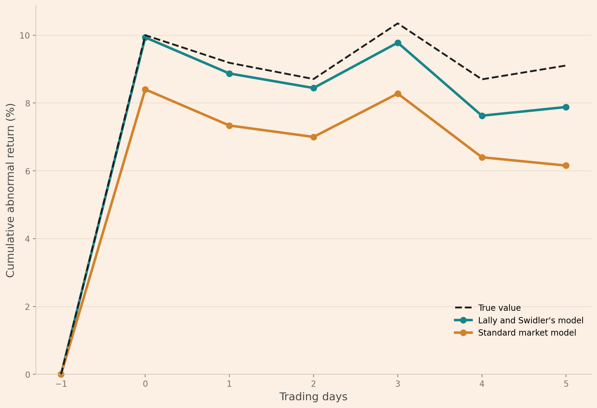
Five trading days after the announcement, the true cumulative abnormal return is 9.1%. Lally and Swidler’s (2003) model gives 7.9%, and the standard market model 6.2%.
Conclusion
Given today’s concentration of large stocks and its history, estimating their abnormal returns, or anything similar, comes with assumptions, and those assumptions can be violated given the nature of the variables one is interested in estimating. I show how to adjust for this violation when dealing with large stocks.
Read next
- Do stocks still drift after earnings announcements?
- Using the Fama-French factors in Python to test a portfolio’s alpha
Disclaimer: a teaching example on simulated data, not investment advice.
References
Lally, M., & Swidler, S. (2003). The effect of an asset’s market weight on its beta: Implications for international markets. Journal of Multinational Financial Management, 13(2), 161–170. https://doi.org/10.1016/S1042-444X(02)00041-5