Does an IPO boom precede a weak year for the S&P 500?
When US initial public offerings (IPOs) over the prior 12 months were at least 3.0% of listed US firms, the S&P 500 total return, with dividends reinvested, over the next 12 months was 2.0 percentage points below its all-months average. At the 7.0% threshold it was 3.5 points above. One argument for a market top is that companies sell shares when prices are high, so a year of many IPOs should precede poor returns. Pastor and Veronesi (2003) find that IPO volume increases with recent market returns and forecasts a lower return the next quarter, a modest negative link through the cost of capital, the return investors require.
I test whether high IPO intensity, many IPOs relative to the number of listed firms, warned of a weak next year for the S&P 500 over the full 1988 to 2025 record. The abnormal return, the next-year return minus its average over all months, was within a few points of zero and changed sign, so high IPO intensity was not a stable warning.
The test
- Signal. IPO intensity is the number of US IPOs over the prior 12 months, divided by the number of listed US firms, as a percent. Deflating by the firm count follows Pastor and Veronesi (2003) and keeps the 1990s comparable to today.
- Universe. Approximate operating-company IPOs on major US exchanges: common shares, an offer price of at least $5, no special-purpose acquisition companies and no business development companies. This keeps 8,117 of 17,584 raw deals.
- Thresholds. Nested thresholds from 1.0% to 7.0% of listed firms. Each keeps the months where intensity had been at least that high, as long as at least 12 such months exist.
- Outcome. The S&P 500 total return over the next 12 months, averaged across the qualifying months, less the all-months average.
- Sample. Signal months from January 1988 to June 2025, so the last forward return ends in mid-2026.
Starting point
The test runs off two files: monthly IPO counts built from an LSEG deal list, and the S&P 500 total-return index. Building them is a separate job that depends on the data vendor. I pull from LSEG Workspace. Because the data is licensed, the raw files stay off this page, and I show the code without running it here. The listed-firm deflator is the World Bank count of domestically listed companies, which is public.
Step 1. The signal
Each month-end I count the IPOs over the prior 12 months, divide by the number of listed US firms, and pair that with the S&P 500 total return over the next 12 months.
# cnt does not necessarily contain every month end that mo does. reindex() puts the missing
# ones back on the shared index, and fillna(0) counts such a month as zero IPOs rather than
# leaving a gap, which would leave the rolling window below with twelve missing readings.
ipos_each_month = cnt.reindex(mo.index).fillna(0)

# rolling(12) adds up the twelve rows ending at each row, so a month's reading uses that
# month and the eleven before it, and nothing that came later.
ipos_prior_12m = ipos_each_month.rolling(12).sum()

signal = ipos_prior_12m / firms * 100        # IPOs as a percent of listed US firms

# shift(-12) pulls the index level from twelve months ahead back onto today's row, so each
# month has, on the same row, the total return earned over the year that followed it.
index_in_12m = mo.shift(-12)
forward_return = index_in_12m / mo - 1

# The first eleven months have no full window behind them and the last twelve have no
# forward return yet. dropna() drops those rows, so every row left has both a signal
# and the outcome that follows it.
panel = pd.DataFrame({"sig": signal, "fwd": forward_return}).dropna()
Here cnt is the monthly IPO count, mo is the month-end total-return index, and firms is the listed-firm count held flat and lagged one month, so the signal uses only information known at the time. The current reading tells me how busy the IPO market is today.
# This reads the signal itself rather than the panel, so it can run past the last month
# with an outcome. A forward return needs a year of hindsight, and a signal is available
# as soon as the month ends. dropna() first, so the last row is the most recent month
# with a reading.
# first, so the last row is the most recent month with a reading.
observed_signal = signal.dropna()
latest_month = observed_signal.index[-1]     # index[-1] is the last date label
latest_reading = observed_signal.iloc[-1]    # iloc[-1] is the last value by position
print(f"latest IPO intensity = {latest_reading:.1f}% (as of {latest_month:%b %Y})")
latest IPO intensity = 2.7% (as of May 2026)IPO intensity today is 2.7%.
Step 2. The abnormal return at each threshold
For each threshold I take the months where intensity had been at least that high, average their next-12-month S&P 500 return, and subtract the average across all months. That difference is the abnormal return: the S&P 500 return after IPO intensity at least that high, relative to a normal year.
MIN_MONTHS = 12          # a threshold is reported only if at least this many months clear it

# The signal months the test runs on, 1988 to 2025. Every row already has the
# return over the twelve months after it, so a month kept here uses data a year further on.
in_sample = (panel.index.year >= 1988) & (panel.index.year <= 2025)
sample = panel[in_sample]

# The benchmark every threshold is measured against: what a month returned over the
# following year on average, whatever the IPO market was doing at the time. Multiplying by
# 100 turns a decimal return into percent.
all_month_average = sample["fwd"].mean() * 100

# The cut-offs the sweep runs, as a percentage of listed US firms over the prior 12 months.
THRESHOLDS = [1.0, 1.5, 2.0, 2.5, 3.0, 3.5, 4.0, 4.5, 5.0, 5.5, 6.0, 6.5, 7.0]

# One pass per threshold. Each keeps the months at or above it, and a threshold left with
# too few months is skipped rather than reported from a handful of overlapping windows.
reported_thresholds = []
abnormal_returns = []

for threshold in THRESHOLDS:
    qualifying = sample[sample["sig"] >= threshold]
    qualifying_months = len(qualifying)        # the months column of the table below
    if qualifying_months < MIN_MONTHS:
        continue

    conditional_average = qualifying["fwd"].mean() * 100
    reported_thresholds.append(threshold)

    # The abnormal return: the average at this threshold, less a normal year
    abnormal_returns.append(conditional_average - all_month_average)
The printed abnormal return at each threshold, with the number of qualifying months:
threshold   months   abnormal return
   1.0%      419         -0.9%
   1.5%      400         -1.0%
   2.0%      340         -0.7%
   2.5%      309         -1.2%
   3.0%      260         -2.0%
   3.5%      204         -1.8%
   4.0%      157         -0.6%
   4.5%      124         -1.0%
   5.0%      112         -0.6%
   5.5%       96         -0.6%
   6.0%       69         -1.3%
   6.5%       48         +0.8%
   7.0%       33         +3.5%
The abnormal return was within a few points of zero at every threshold. The largest negative abnormal return was 2.0 points at the 3.0% threshold, across 260 months. The two most extreme thresholds had a positive abnormal return. At 6.5% it was 0.8 points above average across 48 months. At 7.0% it was 3.5 points above average across 33 months. So, in this sample high IPO intensity was not a stable warning of a weak next year.
Step 3. The chart
fig, ax = plt.subplots(figsize=(9.2, 6.2))
ax.axhline(0, color="#888", lw=1.0)                          # a normal year

# "-o" is matplotlib shorthand for a solid line with a circle drawn at each point
ax.plot(reported_thresholds, abnormal_returns, "-o", color="#d62728", lw=1.9, ms=6.5)

ax.axvline(latest_reading, color="#1a1a1a", ls="--", lw=1.2)     # marks today's IPO intensity
ax.set_xlabel("IPO intensity threshold (% of US firms in prior 12 months)")
ax.set_ylabel("Next-12-month S&P 500 abnormal return (%)")
ax.set_title("Next-12-month S&P 500 abnormal return by IPO intensity threshold, 1988 to 2025")
plt.savefig("post_ipo_rate_threshold_1988.png", dpi=450, bbox_inches="tight")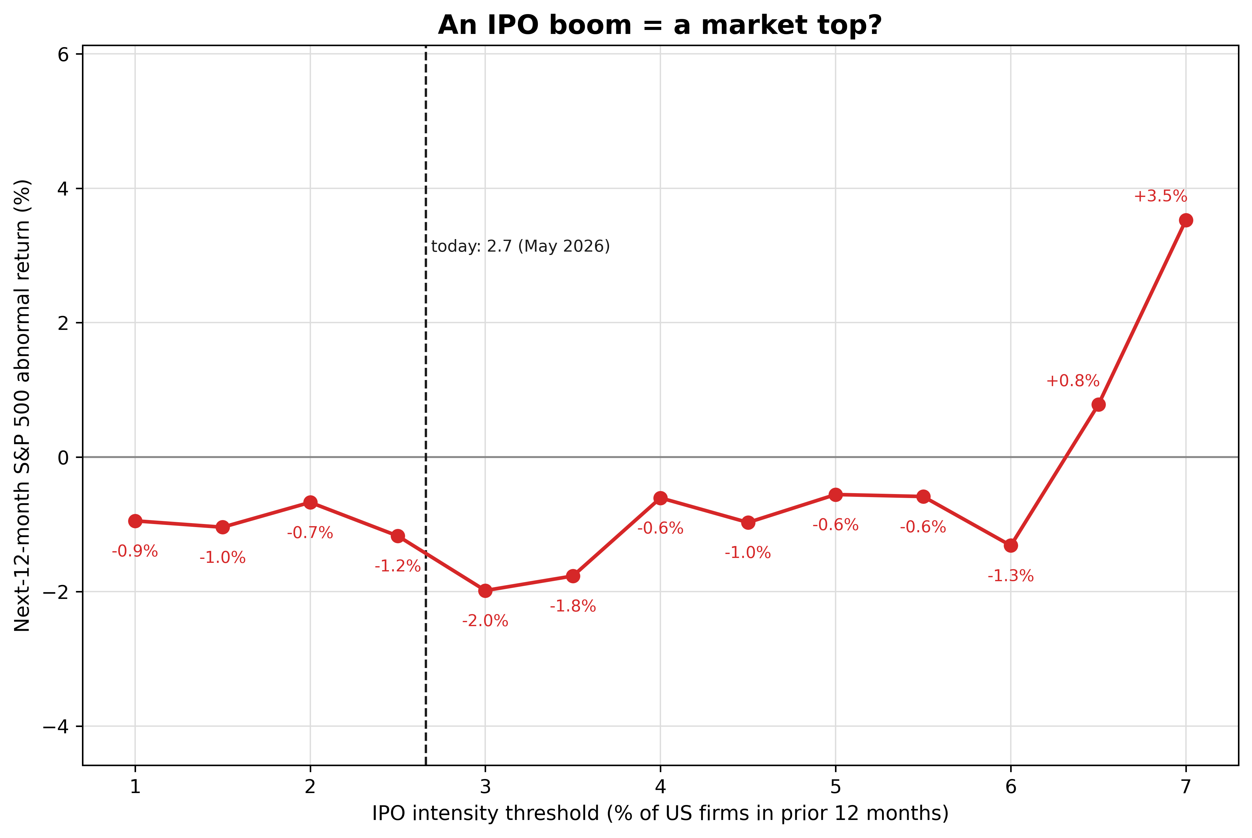
The red line is close to the zero line across the whole range and is above it at the two highest thresholds. The dashed line marks today’s IPO intensity of 2.7%.
Step 4. Which years supply the extreme readings
The positive abnormal returns at the 6.5% and 7.0% thresholds are averages over only 48 and 33 months. To see whether recent booms supply those months, I start the sample in 2000 and list the years with readings at or above 6.0%.
# The 2000-onward sample, checked on its own for which years supply its extreme readings
in_recent_window = (panel.index.year >= 2000) & (panel.index.year <= 2025)
recent_sample = panel[in_recent_window]

for threshold in (6.0, 6.5, 7.0):
    qualifying = recent_sample[recent_sample["sig"] >= threshold]

    # value_counts() counts how many months are in each year, and orders the result by
    # that count, so sort_index() is needed to put the years back into calendar order.
    months_per_year = qualifying.index.year.value_counts().sort_index()

    parts = []
    for year, months in months_per_year.items():
        parts.append(f"{year}: {months} months")
    print(f">= {threshold}%: " + ", ".join(parts))
>= 6.0%: 2000: 9 months, 2021: 7 months
>= 6.5%: 2000: 5 months, 2021: 7 months
>= 7.0%: 2000: 2 months, 2021: 4 monthsIn the 2000-onward window the readings at or above 6.0% come from two periods, the 2000 dot-com peak and the 2021 IPO boom. The years after both booms were weak. Across the full record, the abnormal return at the 6.5% and 7.0% thresholds was positive. Only 12 of the 48 months at 6.5% and 6 of the 33 months at 7.0% are in 2000 or later. So, the positive abnormal return at those two thresholds comes mostly from the months before 2000.
Limitations
Overlapping windows and nested thresholds. The 12-month forward returns of adjacent months share 11 of their 12 months, and each threshold is a subset of the one below it. The months are therefore not independent draws, so I do not attach confidence intervals, ranges that likely contain the true values, to any point. I describe the shape of the line and do not report any single threshold as a result.
The highest thresholds depend on the start year. Most of their months are from before 2000, and their months from 2000 onward come from the 2000 and 2021 booms, which were followed by weak years. A sample that starts later could give those thresholds a different sign, so I do not treat IPO intensity as a stable signal.
An approximate IPO universe. I assign months by LSEG issue date, and the operating-company filter is an approximation. Against Ritter’s net IPO count over 1988 to 2025, the monthly series correlates at 0.973 and totals 1.073 times his count, with a mean absolute monthly difference of 2.9 IPOs. The levels are close enough for a percent-of-firms signal.
A different method from Pastor and Veronesi. They ran quarterly regressions, statistical fits that relate the next quarter’s return to several variables at once, over 1960 to 2002 and found a modest negative link. This is a plain threshold test on the next year’s return over the later 1988 to 2025 sample. It is a reassessment at a different horizon, so it neither reproduces nor refutes their result.
Conclusion
Over the 1988 to 2025 record, the abnormal return was within a few points of zero at every threshold. Its most negative value was 2.0 points below average, at 3.0% of listed firms, and it was positive at the two most extreme thresholds, where most months are from before 2000. In the 2000-onward window the readings at or above 6.0% come from the 2000 and 2021 booms. Selling out because IPOs are booming assumes that IPO intensity predicts next year’s S&P 500 return, and over this sample that prediction was not reliable. The takeaway is that a busy IPO year was not a stable warning of a weak year for the S&P 500, because the abnormal return was near zero and changed sign across thresholds.
Read next
- The priciest profitable IPOs pop 13.2% and then return -2.1% over their first year The other IPO study: what debut size and valuation say about returns.
- Download US IPO data from LSEG Workspace in Python The pipeline that built the IPO counts behind this post.
Disclaimer: this is a simplified, descriptive historical test for discussion purposes only. Not investment advice. Past performance does not guarantee future returns.
Data: US IPO deal records and the S&P 500 total-return index from LSEG Workspace (licensed); listed-firm counts from the World Bank and the validation count from Jay Ritter. Because the LSEG data is licensed, I do not reproduce the raw file here. Pastor and Veronesi (2003) is the source for the firm-count deflator and for the quarterly result this test is compared with.