The priciest profitable IPOs pop 13.2% and then return -2.1% over their first year

Sorted by price-to-earnings ratio at the offer, the cheapest quarter of profitable US IPOs returned a median 13.0% in its first year, against −2.1% for the priciest.

Sorted by the price-to-earnings ratio at the offer, the priciest quarter of profitable US initial public offerings (IPOs) opened a median 13.2 percent above the offer price, the price at which the company sold its shares. Half of them opened more than 13.2 percent above it, and half less. Their median return over the first year was minus 2.1 percent. The cheapest quarter opened 5.3 percent above the offer and returned 13.0 percent. The day-one pop, the rise from the offer price to the opening trade, went to investors allocated shares at the offer, and the first-year return is what a buyer at the day-1 close earned.

The median pop also increases with debut size. Across 2,417 US IPOs from 2000 to July 2025, the smallest fifth by size at the offer opened a median 0.2 percent above the offer and the largest fifth 13.9 percent. In the two fifths below about half a billion dollars at the offer, the median IPO opened close to the offer price, and in the three larger fifths well above it. I sort IPOs into buckets by debut size and by valuation and compare the median pop and the median first-year return across the buckets.

The setup

• Universe: US IPOs, active and delisted, each with a positive offer price, a first-trade opening print, and an IPO deal dated within seven days of the first trade, leaving out uplistings and relistings. I keep the 2,417 that debuted from January 2000 to 24 July 2025, at least one year before the run that produced the tables.
• Size: offer-implied market cap, the day-1 share count repriced at the offer, deflated to 2026 dollars.
• Valuation: offer-implied price-to-earnings (P/E), the offer-priced company over its last reported annual earnings, with loss-makers held as their own bucket.
• Returns: the first-day pop from the offer to the opening trade, then the median return from the day-1 close over the next month and the next year.
• Sample rule: only debuts at least one year old, so the one-year column covers nearly the same companies as every other column. All 2,417 have a pop, 2,405 a one-month return and 2,383 a one-year return. The 34 without a one-year return delisted within their first year, debuted less than a year before I built the data file, or have no return after day one in the file.

Starting point

The analysis uses one file, which I build from LSEG Workspace data in a separate job. Because the data is licensed, the raw file stays off this page, and the code below is shown without being run on this page. The download route is the one from an earlier post, with the field list set to IPO offer prices, opening prints, market caps, and fundamentals.

Step 1. Size at the offer price

The size measure is offer-implied market cap: the share count LSEG used on day one, repriced at the offer price from the night before. Day-1 market cap already contains the pop I am measuring. A stock that pops 100 percent doubles its “size” before the sort, which moves the IPOs with the largest pops into the top bucket and makes size appear to predict the pop. Repricing the same share count at the offer removes that contamination.

NoteCode: the size at the offer price

import pandas as pd

all_ipos = pd.read_csv("ipo_data.csv", parse_dates=["first_trade_date"])

# Offer-implied size: the day-1 share count repriced at the offer.
# Day-1 market cap already contains the pop, so sorting on it would put the
# IPOs with the largest pops into the top buckets and make size appear to predict the pop.
day1_share_count = all_ipos["market_cap_usd"] / all_ipos["day1_close"]
all_ipos["offer_implied_mcap"] = day1_share_count * all_ipos["offer_price"]

# The first-day pop: offer price to the opening trade.
all_ipos["pop_open"] = (all_ipos["day1_open"] / all_ipos["offer_price"] - 1) * 100

# Keep research-grade rows: a real offer, an opening print, a known size, and a
# debut at least a year old, so nearly every IPO kept also has a one-year return.
one_year_ago = pd.Timestamp.now().normalize() - pd.Timedelta(days=365)

# Each test below gives back a column of True and False, one value per IPO.
has_offer_price = all_ipos["offer_price"] > 0
has_opening_print = all_ipos["day1_open"].notna()
has_size = all_ipos["offer_implied_mcap"].notna()
at_least_one_year_old = all_ipos["first_trade_date"] <= one_year_ago

# & keeps only the rows where all four hold. .copy() gives the sample its own memory,
# so the columns added below are written to it and not to a view of all_ipos.
research_grade = (has_offer_price & has_opening_print
                  & has_size & at_least_one_year_old)
sample = all_ipos[research_grade].copy()

An IPO from six months ago has no one-year return yet, so the code keeps only debuts at least a year before the date of the run. The tables below come from a run on 24 July 2026, so they keep debuts up to 24 July 2025. The data file was built on 12 June 2026, so the six IPOs that debuted after 12 June 2025 have no one-year return, and a later run on the same file would add more IPOs without one.

The notebook that produced the tables applies three tests the code on this page leaves out. It drops IPOs whose deal is dated more than seven days from the first trade, drops uplistings and relistings, and computes a P/E only where the earnings and trading currencies match. Without the first two tests, the code above keeps 2,855 IPOs in place of 2,417.

Step 2. Same dollars, five buckets

A 500-million-dollar IPO in 2000 was a bigger company than a 500-million-dollar IPO in 2024, because a dollar bought more then. Without an inflation adjustment, the small bucket would fill with old IPOs and the large bucket with recent ones, so a sort on size would also be a sort on era. I deflate every debut size to 2026 dollars with annual consumer-price index (CPI) factors, then cut the ranked sizes into five equal-count buckets.

NoteCode: the five size buckets

# A $500m IPO in 2000 was a bigger company than a $500m IPO in 2024, because a
# dollar bought more then. Deflate every debut size to 2026 dollars before sorting.
BASE_YEAR = 2026


def inflation_factor(year):
    """Multiplier that restates dollars of `year` in BASE_YEAR dollars."""
    return CPI[BASE_YEAR] / CPI[year]        # CPI maps a year to its price index level


sample["year"] = sample["first_trade_date"].dt.year

# map calls the function once for every value in the column.
sample["cpi_factor"] = sample["year"].map(inflation_factor)
sample["real_mcap"] = sample["offer_implied_mcap"] * sample["cpi_factor"]

# Rank by real size and cut the ranks into five equal-count buckets.
size_labels = ["Q1 smallest", "Q2", "Q3", "Q4", "Q5 largest"]
sample["size_q"] = pd.qcut(sample["real_mcap"], 5, labels=size_labels)

I use qcut, which cuts the ranks into equal-count buckets, because IPO sizes are heavily skewed and a range cut would put nearly every IPO in the bottom bucket. The buckets contain about 484 IPOs each, with a median size of 129.3 million dollars in Q1 and 4.2 billion in Q5.

Step 3. What each size bucket returned

I report the median, because IPO outcomes have long right tails and the median is what the typical IPO in the bucket did. The one-month and one-year returns start at the day-1 close, so they leave out both the pop and the day-one open-to-close return. For one IPO the three returns chain: one plus the pop, times one plus the open-to-close return, times one plus the one-year return, gives one plus the return from the offer price. The medians of the three columns do not chain in the same way.

NoteCode: the returns of each size bucket

# apply hands this function one bucket of IPOs at a time. Returning a Series turns its
# keys into the columns of the table, in the order they are written here.
def bucket_stats(bucket):
    """Summarise one bucket of IPOs as a single row of counts and medians."""
    # Set aside the IPOs that have a one-year return, so that a missing return stays out
    # of the up_1y_% share instead of counting as an IPO that finished down.
    one_year_returns = bucket["ret_1y_pct"].dropna()

    return pd.Series({
        "n": len(bucket),
        "size_med_$m": bucket["real_mcap"].median() / 1e6,   # 1e6 turns dollars into millions
        "pop_%": bucket["pop_open"].median(),
        "ret_1m_%": bucket["ret_1m_pct"].median(),   # both returns are measured from the
        "ret_1y_%": bucket["ret_1y_pct"].median(),   # day-1 close, so after the pop
        "up_1y_%": (one_year_returns > 0).mean() * 100,   # mean of True and False is a share
    })


# observed=True reports only the buckets that contain IPOs.
size_table = sample.groupby("size_q", observed=True).apply(bucket_stats).round(1)

             n   size_med_$m   pop_%   ret_1m_%   ret_1y_%   up_1y_%
Q1 smallest  484       129.3     0.2       -1.4      -14.8      36.1
Q2           483       374.3     3.5        1.9        1.9      51.9
Q3           483       654.7    10.7        1.5       -6.3      43.7
Q4           483      1261.2    12.7        2.5        1.8      51.8
Q5 largest   484      4227.9    13.9        1.8       -8.2      43.8

In the table, n is the number of IPOs in a bucket, size_med_$m their median size in millions of dollars, pop_% the median pop, ret_1m_% and ret_1y_% the median one-month and one-year returns from the day-1 close, all in percent, and up_1y_% the share of the bucket that finished the year above the day-1 close. The median pop is 0.2 percent in the smallest bucket and 3.5 percent in the second, then 10.7, 12.7 and 13.9 percent in the three largest, with median sizes from 654.7 million dollars up. The median one-month returns are small in every bucket, from −1.4 to 2.5 percent.

The median first-year return did not increase with debut size: minus 14.8 percent in the smallest fifth, the worst of the five, where only 36.1 percent finished above the day-1 close, then 1.9, minus 6.3 and 1.8 percent, and minus 8.2 percent in the largest fifth.

Median first-day pop, day-one open-to-close, one-month and one-year return for US IPOs, sorted into five buckets by inflation-adjusted offer-implied size.

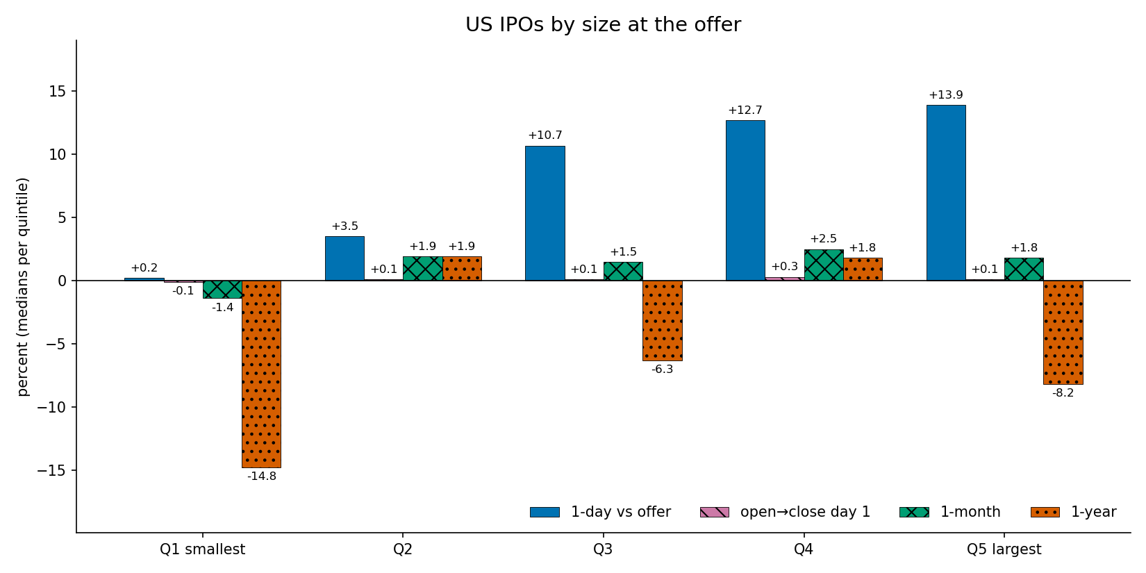
The pop went to investors allocated shares at the offer. A buyer at the opening trade earned a median of close to nothing on day one. The day-one open-to-close bars in the chart above are close to zero in every size bucket.

Step 4. Sort by valuation instead

Next, I sort the same IPOs by the offer-implied P/E. The P/E uses the offer price, for the same reason as the size measure: the pop does not leak into the valuation. Loss-makers get their own bucket, because a P/E is defined only for a company with positive earnings, and they are the majority of the sample.

NoteCode: the valuation buckets

import numpy as np

# Offer-implied P/E: the offer-priced company over its last reported annual earnings.
# A P/E is defined only when the company earned money, so the ratio is left missing
# for the loss-makers, and they get a bucket of their own below.
profitable = sample["net_income_fy0"] > 0
offer_value = sample.loc[profitable, "offer_implied_mcap"]
earnings = sample.loc[profitable, "net_income_fy0"]

sample["pe_offer"] = np.nan                    # every IPO starts with no P/E
sample.loc[profitable, "pe_offer"] = offer_value / earnings

# Loss-makers are their own bucket; the profitable split into four P/E quartiles.
# NaN <= 0 is False, so a company with no earnings record joins neither group and drops
# out of the table, which is how the names without usable earnings leave the sort.
loss_making = sample["net_income_fy0"] <= 0
has_pe = sample["pe_offer"].notna()

# valuation_q holds the valuation bucket. Assigning into a column that does not exist yet creates
# it, and leaves NaN wherever the mask is False.
pe_labels = ["P/E Q1 cheapest", "P/E Q2", "P/E Q3", "P/E Q4 priciest"]
sample.loc[loss_making, "valuation_q"] = "Loss-making"
sample.loc[has_pe, "valuation_q"] = pd.qcut(sample.loc[has_pe, "pe_offer"], 4, labels=pe_labels)

has_valuation_bucket = sample["valuation_q"].notna()
valuation_sample = sample[has_valuation_bucket]
pe_table = valuation_sample.groupby("valuation_q", observed=True).apply(bucket_stats).round(1)

Of the 2,417 IPOs, 1,289 were loss-making at the offer, 909 were profitable with a usable P/E, and 219 dropped out with no earnings record or a currency mismatch, mostly funds and shell companies. The table below shows each bucket’s median offer-implied P/E, pe_med, in place of the median size column, left empty (NaN) for the loss-makers, which have no P/E. bucket_stats above computes the median size, and the run that produced this table put the median of pe_offer in that column instead.

                    n   pe_med   pop_%   ret_1m_%   ret_1y_%   up_1y_%
Loss-making      1289      NaN     9.4       -0.3      -20.6      37.5
P/E Q1 cheapest   228     10.1     5.3        3.5       13.0      65.5
P/E Q2            227     23.6     8.3        3.3       11.6      60.2
P/E Q3            227     49.4     8.8        3.7        3.6      53.3
P/E Q4 priciest   227    167.6    13.2        2.6       -2.1      48.0

Among the profitable IPOs, the median first-year return decreases as the offer P/E increases. The cheapest quarter, at a median P/E of 10.1, returned a median 13.0 percent, and 65.5 percent of them finished up. The median first-year return is 11.6 percent in P/E Q2, 3.6 percent in P/E Q3, and minus 2.1 percent in the priciest quarter, at a median P/E of 167.6. The loss-makers, just over half the sample, lost the most at 20.6 percent, and only 37.5 percent of them finished up, even though they popped a median 9.4 percent on day one.

Median first-day pop, day-one open-to-close, one-month and one-year return for US IPOs, split into loss-makers and four offer-implied P/E buckets.

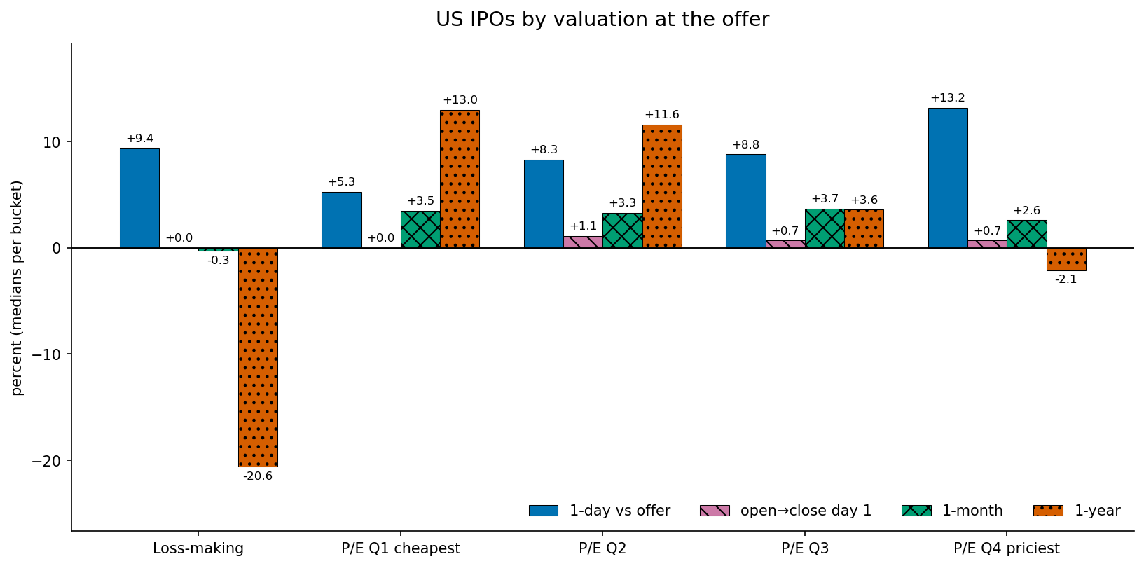
The priciest quarter and the loss-makers had the two largest median pops, 13.2 and 9.4 percent, and the two lowest median first-year returns. So, the two groups in which buyers at the open paid the largest median premium over the offer also had the two lowest median first-year returns.

Limitations

• These are raw returns. I report each IPO’s own return from the day-1 close, without subtracting the market over the same window. A minus 14.8 percent year is a larger shortfall against the market when the market rose than when it fell, so setting each return against the S&P 500 total return, dividends included, over the identical window is a separate test and is not in this post.
• Some delisted names are missing from the sample. The sample keeps delisted IPOs where the vendor file contains their listing dates, and drops the ones where it does not. I have not measured how many are missing or how their absence changes the medians.
• One specification, pooled across 26 years. The size buckets pool every IPO from 2000 to July 2025, and the 2025 and 2026 CPI values are estimates. The bucket edges and the P/E cut are choices, and I do not attach a confidence interval, a range that likely contains the true value, to any single number.
• The P/E uses pre-IPO earnings. I compute the P/E from the last reported annual earnings before the IPO, only where the filing and trading currency match. The 219 names without a usable earnings record drop out of the valuation cut.

Conclusion

The median pop is higher in the larger size buckets, and among profitable IPOs the median first-year return is lower in the pricier P/E buckets. The takeaway is that the largest median pops came with large or expensive deals, and among profitable IPOs the cheapest quarter had the highest median first-year return.

Read next

• Does an IPO boom precede a weak year for the S&P 500? The other IPO study: whether a busy IPO year warns of weak market returns.
• Download US IPO data from LSEG Workspace in Python How to download the IPOs of US issuers from LSEG’s deals database.

Disclaimer: a simplified, descriptive study for discussion purposes only. Not investment advice. Past performance does not guarantee future returns.

Data: US IPO offer prices, opening prints, market caps, and fundamentals from LSEG Workspace (licensed). I do not reproduce the raw file here.