The Markowitz curse
Suppose we want to choose the weights of two stocks in a portfolio so that the portfolio has the lowest possible volatility. These weights, the minimum-variance weights, follow from a textbook formula that uses the two stocks’ volatilities and their correlation, estimated from past returns.
When the correlation is high, the weights depend heavily on these estimates. At a correlation of 0.99, two stocks that both have an estimated volatility of 20% get 50% weight each. But if one stock’s estimated volatility is 0.2 percentage points higher, the other stock gets 99.5% weight. At a correlation of 0.5, the same difference changes the weights only to 51/49.
The problem is that we never know the volatilities exactly. We estimate them from past returns, and even if both stocks truly have a volatility of 20%, five years of returns give each stock an estimated volatility a little above or below 20%, by chance. In 1,000 simulated samples of five years of monthly returns for two such stocks, at a true correlation of 0.99, the minimum-variance weights computed from these estimates give one stock 100% weight in 60.0% of the samples, although the true minimum-variance weights are 50/50.
The same instability can occur with many stocks, and two stocks make its mechanism easiest to see. López de Prado (2016) calls it Markowitz’s curse and proposes a method, hierarchical risk parity, that Step 5 tests with four stocks.
Step 1. Computing the minimum-variance weight
Step 1 shows why a 0.2-point difference between the estimated volatilities changes the weight so much at a correlation of 0.99. The formula for the minimum-variance weight in stock A, Equation 5.9 in Elton, Gruber, Brown and Goetzmann (2014), can be written as
\[\begin{aligned} w_A &= \frac{1}{2} + \frac{\sigma_B^2 - \sigma_A^2}{2\operatorname{Var}(R_A - R_B)},\\ \operatorname{Var}(R_A - R_B) &= (\sigma_A - \sigma_B)^2 + 2(1 - \rho)\,\sigma_A\sigma_B, \end{aligned}\]
where \(\sigma_A\) and \(\sigma_B\) are the two stocks’ volatilities, so \(\sigma_A^2\) and \(\sigma_B^2\) are their variances, \(\rho\) is their correlation, and \(R_A - R_B\) is the difference between their returns. Stock B’s weight is 100% minus stock A’s.
When the two stocks move almost together, their returns differ little from month to month, so the variance of the difference between the returns is small. Dividing by it turns a small difference between the variances into a large change in the weight.
With stock A’s estimated volatility at 20% and stock B’s at 20.2%, written in percent, the difference between the variances is \(20.2^2 - 20^2 = 8.04\), and the first term of \(\operatorname{Var}(R_A - R_B)\) is \((20 - 20.2)^2 = 0.04\). Neither number depends on the correlation. At a correlation of 0.5,
\[\begin{aligned} \operatorname{Var}(R_A - R_B) &= 0.04 + 2(1 - 0.5)(20)(20.2)\\ &= 404.04,\\ w_A &= 0.5 + \frac{8.04}{2 \times 404.04} = 51.0\%, \end{aligned}\]
and at 0.99,
\[\begin{aligned} \operatorname{Var}(R_A - R_B) &= 0.04 + 2(1 - 0.99)(20)(20.2)\\ &= 8.12,\\ w_A &= 0.5 + \frac{8.04}{2 \times 8.12} = 99.5\%. \end{aligned}\]
Only \(1 - \rho\) differs between the two cases. It is 0.5 at a correlation of 0.5 and 0.01 at 0.99, which makes the second term of \(\operatorname{Var}(R_A - R_B)\) 404 in the first case and 8.08 in the second. So the same 8.04 is divided by \(2 \times 404.04 = 808.08\) at a correlation of 0.5 and by \(2 \times 8.12 = 16.24\) at 0.99.
The formula can also give a weight below 0% or above 100%, which would mean selling one stock short. As in López de Prado’s (2016) comparison, I do not allow short sales: a weight below 0% becomes 0%, and one above 100% becomes 100%. The block below computes the weight, with the volatilities in percent, for stock B’s estimated volatility at 19.8%, 20.0% and 20.2%, at both correlations.
import matplotlib.pyplot as plt
import numpy as np
import pandas as pd

# One row per case: stock A's estimated volatility at 20%, and stock B's at 19.8%, 20.0% or
# 20.2%, at a correlation of 0.5 and of 0.99, with the volatilities in percent
cases = pd.DataFrame({
    "correlation": [0.5, 0.5, 0.5, 0.99, 0.99, 0.99],
    "volatility A (%)": 20.0,
    "volatility B (%)": [19.8, 20.0, 20.2, 19.8, 20.0, 20.2]})

# The formula above, on every row at once: the difference between the variances, stock B's minus
# stock A's, the variance of the difference between the returns, Var(R_A - R_B), and the weight
# in stock A. clip(0, 1) moves a weight below 0 up to 0 and one above 1 down to 1, as there are
# no short sales
cases["difference between the variances"] = (cases["volatility B (%)"]**2
                                             - cases["volatility A (%)"]**2)
cases["variance of the difference"] = ((cases["volatility A (%)"] - cases["volatility B (%)"])**2
                                       + 2 * (1 - cases["correlation"])
                                       * cases["volatility A (%)"] * cases["volatility B (%)"])
cases["weight in A (%)"] = 100 * (0.5 + cases["difference between the variances"]
                                  / (2 * cases["variance of the difference"])).clip(0, 1)
# The inputs and the weight, with the weight rounded to one decimal; index=False leaves out the
# row numbers
print(cases[["correlation", "volatility A (%)", "volatility B (%)", "weight in A (%)"]]
      .round({"weight in A (%)": 1}).to_string(index=False))
correlation volatility A (%) volatility B (%) weight in A (%)
0.50 20.0 19.8 49.0
0.50 20.0 20.0 50.0
0.50 20.0 20.2 51.0
0.99 20.0 19.8 0.0
0.99 20.0 20.0 50.0
0.99 20.0 20.2 99.5At a correlation of 0.5, the weight in stock A is between 49.0% and 51.0%. At 0.99, it changes from 0% to 99.5% while stock B’s estimated volatility changes by 0.4 points.
Step 2. Plotting the weight against stock B’s estimated volatility
Step 2 shows how steeply the weight changes between these cases. The chart plots the weight, computed with the same formula as in Step 1, for every estimated volatility of stock B from 19.8% to 20.2%, with stock A’s at 20%.
BG, INK, GRID, SPINE, AXIS_TEXT = "#FCEFE3", "#1f1f1f", "#EADCCC", "#D5C6B4", "#4a4a4a"
TEAL, GREY = "#17868A", "#888888"

# One row per correlation and estimated volatility of stock B, with stock A's at 20%:
# np.linspace(19.8, 20.2, 401) gives 401 evenly spaced values from 19.8% to 20.2%, and merge with
# how="cross" pairs every correlation with every volatility
grid = (pd.DataFrame({"correlation": [0.99, 0.5]})
        .merge(pd.DataFrame({"volatility B (%)": np.linspace(19.8, 20.2, 401)}), how="cross"))
grid["volatility A (%)"] = 20.0
# The same formula as in Step 1, on every row at once
grid["difference between the variances"] = (grid["volatility B (%)"]**2
                                            - grid["volatility A (%)"]**2)
grid["variance of the difference"] = ((grid["volatility A (%)"] - grid["volatility B (%)"])**2
                                      + 2 * (1 - grid["correlation"])
                                      * grid["volatility A (%)"] * grid["volatility B (%)"])
grid["weight in A (%)"] = 100 * (0.5 + grid["difference between the variances"]
                                 / (2 * grid["variance of the difference"])).clip(0, 1)
# The rows of each correlation: .loc[condition] keeps the rows where the condition is True
line_099 = grid.loc[grid["correlation"] == 0.99]
line_05 = grid.loc[grid["correlation"] == 0.5]

# The figure and its chart, 10 by 6 inches; lw is the line width, and label is the legend's text
fig, axis = plt.subplots(figsize=(10, 6))
axis.plot(line_099["volatility B (%)"], line_099["weight in A (%)"], color=TEAL, lw=2.8,
          label="Correlation 0.99")
axis.plot(line_05["volatility B (%)"], line_05["weight in A (%)"], color=GREY, lw=2.8,
          label="Correlation 0.5")
# The weight at both ends of each line: iloc[0] is the first row and iloc[-1] the last, and
# {:.1f} writes one decimal. annotate puts each label 6 points to the side and 12 points below
# the left end or above the right end, where a point is 1/72 inch
start_099 = line_099["weight in A (%)"].iloc[0]
end_099 = line_099["weight in A (%)"].iloc[-1]
start_05 = line_05["weight in A (%)"].iloc[0]
end_05 = line_05["weight in A (%)"].iloc[-1]
axis.annotate(f"{start_099:.1f}%", (19.8, start_099), xytext=(6, -12),
              textcoords="offset points", va="center", color=TEAL, fontsize=13)
axis.annotate(f"{end_099:.1f}%", (20.2, end_099), xytext=(-6, 12),
              textcoords="offset points", ha="right", va="center", color=TEAL, fontsize=13)
axis.annotate(f"{start_05:.1f}%", (19.8, start_05), xytext=(6, -12),
              textcoords="offset points", va="center", color=GREY, fontsize=13)
axis.annotate(f"{end_05:.1f}%", (20.2, end_05), xytext=(-6, 12),
              textcoords="offset points", ha="right", va="center", color=GREY, fontsize=13)
# A dot (ms is its size) where both estimated volatilities are 20% and the weight is 50%
axis.plot(20.0, 50, "o", color=INK, ms=8, zorder=3)
axis.annotate("Both estimated volatilities 20%: 50/50", (20.0, 50), xytext=(12, -16),
              textcoords="offset points", va="center", color=INK, fontsize=12)
axis.set_xlim(19.8, 20.2)
axis.set_ylim(-10, 108)
axis.set_xticks([19.8, 19.9, 20.0, 20.1, 20.2])
axis.set_yticks([0, 25, 50, 75, 100])
axis.set_xlabel("Stock B's estimated volatility (%), with stock A's at 20%", fontsize=12,
                color=AXIS_TEXT)
axis.set_ylabel("Minimum-variance weight in stock A (%)", fontsize=12, color=AXIS_TEXT)
# The legend in the empty top left, without a frame, each entry in its line's colour
axis.legend(loc="upper left", frameon=False, fontsize=13, labelcolor="linecolor")
# The site's chart style: the background colour, a light grid on the y-axis only, drawn behind
# the lines, no top and right borders, and tick labels without tick marks (length=0)
fig.patch.set_facecolor(BG)
axis.set_facecolor(BG)
axis.grid(True, axis="y", color=GRID)
axis.set_axisbelow(True)
axis.spines[["top", "right"]].set_visible(False)
axis.spines[["left", "bottom"]].set_color(SPINE)
axis.tick_params(axis="both", length=0, colors=INK, pad=6)
plt.savefig("markowitz_curse.png", dpi=150, bbox_inches="tight", facecolor=BG)
plt.show()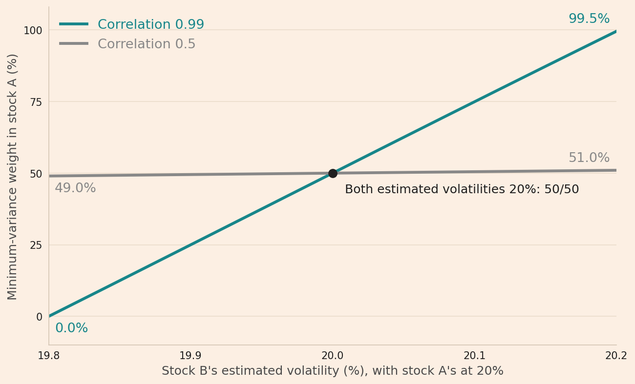
The grey line, for a correlation of 0.5, is almost flat. The teal line, for 0.99, increases from 0% to 99.5% and crosses the grey line at 50%, where both estimated volatilities are 20%.
Step 3. Simulating the returns
So far, I set the estimated volatilities by hand. In practice, they differ from the true volatilities by chance, because they come from a limited number of past returns. They can also be out of date, because “characteristics of security returns usually change over time” (Elton, Gruber, Brown and Goetzmann, 2014, p. 87).
Step 3 simulates a market whose true volatilities and correlation never change, to show that the estimated weights change from one sample to the next even then.
- Returns. Each month, each stock’s return is an assumed average of 0.7% plus a random part. The random parts have a true volatility of 20% a year for both stocks and the true correlation between them.
- True correlations. 0.5 or 0.99.
- Samples. 1,000 samples per true correlation, each of 60 monthly returns ending in September 2026.
- True weights. Both stocks have the same true volatility, so the true minimum-variance weight is 50% in every sample.
Each month \(t\), the two returns are
\[\begin{aligned} r_{A,t} &= \mu + s\,z_{1,t},\\ r_{B,t} &= \mu + s\left(\rho\,z_{1,t} + \sqrt{1 - \rho^2}\,z_{2,t}\right), \end{aligned}\]
where \(\mu = 0.7\%\) is the monthly average, which the weights do not use, \(s = 20\%/\sqrt{12} = 5.77\%\) the monthly volatility, \(\rho\) the true correlation, and \(z_{1,t}\) and \(z_{2,t}\) independent draws from the standard normal distribution, with an average of 0 and a standard deviation of 1. Stock B’s random part has the variance \(s^2(\rho^2 + 1 - \rho^2) = s^2\), the same as stock A’s, and its covariance with stock A is \(s^2\rho\), so the correlation is \(\rho\). The panel has one row per true correlation, sample and month, \(2 \times 1{,}000 \times 60 = 120{,}000\) rows, and every row has draws of its own.
VOLATILITY = 0.20                    # sigma, each stock's true annual volatility
MONTHLY_VOLATILITY = VOLATILITY / np.sqrt(12)                      # s, the monthly volatility
MONTHLY_MEAN = 0.007                 # mu, an assumed 0.7% a month; the weights do not use it
MONTHS = pd.date_range(end="2026-09-30", periods=60, freq="ME")    # 60 month ends

# One row per true correlation, sample and month: merge with how="cross" pairs every row of one
# table with every row of the other, so the panel has 2 x 1,000 x 60 rows. range(1, 1001) gives
# the sample numbers 1 to 1,000, because a range stops before its end
panel = (pd.DataFrame({"true correlation": [0.5, 0.99]})
         .merge(pd.DataFrame({"sample": range(1, 1001)}), how="cross")
         .merge(pd.DataFrame({"date": MONTHS}), how="cross"))

# Two independent draws per row, z1 and z2, from the standard normal distribution. Stock B takes
# the true correlation times z1 plus the square root of 1 minus its square times z2, so that it
# has stock A's volatility and the true correlation with it
rng = np.random.default_rng(seed=7)
z1 = rng.standard_normal(len(panel))
z2 = rng.standard_normal(len(panel))
panel["return A"] = MONTHLY_MEAN + MONTHLY_VOLATILITY * z1
panel["return B"] = MONTHLY_MEAN + MONTHLY_VOLATILITY * (
    panel["true correlation"] * z1 + np.sqrt(1 - panel["true correlation"]**2) * z2)
The block below shows the number of rows and the first rows of the panel, with the returns as fractions.
# The number of rows, where {:,} writes commas between thousands, and the panel's first five
# rows, with the returns rounded to four decimals
print(f"{len(panel):,} rows; the first five:")
print(panel.head().round(4).to_string(index=False))
120,000 rows; the first five:
true correlation sample date return A return B
0.5 1 2021-10-31 0.0071 -0.1023
0.5 1 2021-11-30 0.0242 0.0184
0.5 1 2021-12-31 -0.0088 -0.0124
0.5 1 2022-01-31 -0.0444 -0.0812
0.5 1 2022-02-28 -0.0193 0.0674Each row is one month of one sample at one true correlation.
Step 4. Estimating the weights from each sample
Step 4 measures how much the weights vary when the volatilities are estimated from each sample, and whether the portfolios formed with those weights have a higher true volatility. From each sample’s 60 months, I estimate the variance of each stock’s return and the variance of the difference between the two returns, multiply them by 12 to make them annual, and compute the weight in stock A with the formula of Step 1, without short sales.
To compare the portfolios, I compute the true volatility of each sample’s portfolio from the true values:
\[\sigma_p = \sigma\sqrt{w^2 + (1 - w)^2 + 2w(1 - w)\rho},\]
where \(w\) is the weight in stock A, \(\sigma = 20\%\) is both stocks’ true volatility, and \(\rho\) is the true correlation. This is the volatility of a two-stock portfolio when both stocks have the volatility \(\sigma\). At \(\rho = 0.99\), it is 19.95% at \(w = 50\%\) and 20.00% at \(w = 0\%\) or \(100\%\), so every weight gives a true volatility between these two values.
# The difference between the two returns in each month, R_A - R_B in the formula
panel["return A minus B"] = panel["return A"] - panel["return B"]

# Each sample's annual variances: var() is the variance within each group of rows, and
# multiplying a monthly variance by 12 makes it annual. reset_index() turns the true correlation
# and the sample back into columns
grouped = panel.groupby(["true correlation", "sample"])
estimates = pd.DataFrame({
    "variance A": grouped["return A"].var() * 12,
    "variance B": grouped["return B"].var() * 12,
    "variance of the difference": grouped["return A minus B"].var() * 12}).reset_index()

# The weight in stock A from the formula of Step 1 with the estimated variances; clip(0, 1)
# moves a weight below 0 up to 0 and one above 1 down to 1, as there are no short sales
estimates["weight in A"] = (0.5 + (estimates["variance B"] - estimates["variance A"])
                            / (2 * estimates["variance of the difference"])).clip(0, 1)
# The absolute difference between the two estimated volatilities, the square roots of the
# variances, and whether the weight gives one stock 100%, a weight of 0 or 1
estimates["absolute difference between the estimated volatilities"] = (
    np.sqrt(estimates["variance B"]) - np.sqrt(estimates["variance A"])).abs()
estimates["100% in one stock"] = (estimates["weight in A"] == 0) | (estimates["weight in A"] == 1)
# The true volatility of the portfolio formed with each sample's weight, from the formula above
# with the true values
weight = estimates["weight in A"]
estimates["true volatility"] = VOLATILITY * np.sqrt(
    weight**2 + (1 - weight)**2 + 2 * weight * (1 - weight) * estimates["true correlation"])

# For each true correlation, one column: the average absolute difference between the estimated
# volatilities, the 5th and 95th percentiles of the weight, between which lie 90% of the
# samples, the share of samples with 100% weight in one stock, and the average true volatility
# against the lowest possible, at 50/50, where the formula gives sigma times the square root of
# (1 + rho) / 2
grouped = estimates.groupby("true correlation")
minimum_variance_summary = pd.DataFrame({
    "absolute difference between the estimated volatilities (points)":
        grouped["absolute difference between the estimated volatilities"].mean() * 100,
    "weight in A, 5th percentile (%)": grouped["weight in A"].quantile(0.05) * 100,
    "weight in A, 95th percentile (%)": grouped["weight in A"].quantile(0.95) * 100,
    "samples with 100% weight in one stock (%)": grouped["100% in one stock"].mean() * 100,
    "true volatility, average (%)": grouped["true volatility"].mean() * 100})
minimum_variance_summary["lowest possible volatility (%)"] = VOLATILITY * np.sqrt(
    (1 + minimum_variance_summary.index) / 2) * 100
# One column per true correlation: T turns the rows into columns, and rename_axis(columns=None)
# leaves the name "true correlation" out of the header row, which then shows the two values only
table = minimum_variance_summary.T.round(2).rename_axis(columns=None)
table_text = table.to_string()
# A line above the table with "true correlation" centred over the two columns. index.str.len()
# counts the characters of each row label and max() takes the longest; splitlines()[0] is the
# table's first line; " " * n repeats a space n times; and center(width) adds spaces on both
# sides of the words up to that width
label_width = table.index.str.len().max()
table_width = len(table_text.splitlines()[0])
print("Minimum-variance weights estimated from 1,000 samples per true correlation:")
print(" " * label_width + "true correlation".center(table_width - label_width))
print(table_text)
Minimum-variance weights estimated from 1,000 samples per true correlation:
true correlation
0.50 0.99
absolute difference between the estimated volatilities (points) 1.80 0.30
weight in A, 5th percentile (%) 31.03 0.00
weight in A, 95th percentile (%) 69.11 100.00
samples with 100% weight in one stock (%) 0.00 60.00
true volatility, average (%) 17.47 19.99
lowest possible volatility (%) 17.32 19.95At a true correlation of 0.99, the two estimated volatilities differ by 0.30 points in the average sample, although the true ones are equal. That is more than the 0.2 points that changed the weight from 50% to 99.5% in Step 1. In 60.0% of the samples, one stock gets 100% weight. At 0.5, the estimated volatilities differ by more, 1.80 points, but the weight changes less: in 90% of the samples, it is between 31.0% and 69.1%.
The true volatility of the portfolios formed with these weights averages 19.99% at 0.99, against 19.95% for the 50/50 portfolio. Both results have one cause: at a true correlation of 0.99, every weight gives almost the same true volatility, between 19.95% and 20.00%. So a small difference between the estimated volatilities is enough to change which weight has the lowest estimated volatility, and a weight far from 50% increases the true volatility only slightly.
Step 5. Using hierarchical risk parity
Step 5 tests the method López de Prado (2016) proposes, hierarchical risk parity. It groups the stocks that move together, splits the portfolio’s weight between the groups in inverse proportion to their variances, and then splits each group’s weight between its stocks in the same way. So it never divides by the variance of a difference between returns. With two stocks, each group holds one stock, so I add two stocks, C and D, to show how the method treats groups.
Stocks A and B keep their correlation of 0.99, stocks C and D have a correlation of 0.6, as two stocks in one industry can have, and each stock in A–B has a correlation of 0.3 with each stock in C–D. All four have a true volatility of 20%. I keep the example to four stocks so that every number is visible. With many stocks, the groups come from a clustering of the correlations, and the same splits repeat within each group.
Here, I set the groups by hand as the pairs A–B and C–D, the same two groups that a clustering of these correlations gives. Within each pair, each stock’s weight is in proportion to one over its variance, an inverse-variance weight. Each pair’s variance follows from those weights, and the pair with the lower variance gets the higher weight:
\[\begin{aligned} w_{A|AB} &= \frac{1/\sigma_A^2}{1/\sigma_A^2 + 1/\sigma_B^2},\\ V_{AB} &= w_{A|AB}^2\,\sigma_A^2 + w_{B|AB}^2\,\sigma_B^2 + 2\,w_{A|AB}\,w_{B|AB}\,\rho_{AB}\,\sigma_A\sigma_B,\\ w_{AB} &= \frac{V_{CD}}{V_{AB} + V_{CD}},\\ w_A &= w_{AB}\,w_{A|AB}, \end{aligned}\]
where \(w_{A|AB}\) is stock A’s weight within the pair A–B, \(w_{B|AB} = 1 - w_{A|AB}\) is stock B’s, \(V_{AB}\) is the pair’s variance, \(\rho_{AB} = 0.99\) is its correlation, and \(w_{AB}\) is the pair’s weight in the portfolio. The pair C–D follows the same formulas, with the weight \(1 - w_{AB}\).
With all four estimated volatilities at 20%, written in percent, the inverse-variance weights within each pair are 50%, so the pairs’ variances are
\[\begin{aligned} V_{AB} &= 0.25(400) + 0.25(400) + 2(0.25)(0.99)(400) = 398,\\ V_{CD} &= 0.25(400) + 0.25(400) + 2(0.25)(0.6)(400) = 320. \end{aligned}\]
The pair A–B gets the weight \(320/(398 + 320) = 44.6\%\), so stocks A and B get 22.3% each, and stocks C and D 27.7% each. The pair whose stocks move more closely together has the higher variance, so it gets the lower weight.
For comparison, the block below also computes the minimum-variance weights of the four stocks, without short sales, from their covariance matrix, as the box explains. It computes both sets of weights with stock B’s estimated volatility at 20.0% and at 20.2%, the other three at 20%, and the true volatility of each portfolio from the true volatilities of 20%.
When short sales are allowed and the covariance matrix is invertible, the minimum-variance weights of several stocks, which add up to 100%, are
\[w = \frac{\Sigma^{-1}\mathbf{1}}{\mathbf{1}^\top\Sigma^{-1}\mathbf{1}},\]
where \(\Sigma\) is the covariance matrix of the stocks’ returns, \(\Sigma^{-1}\) its inverse and \(\mathbf{1}\) a column of ones. For two stocks, this gives the formula of Step 1.
In this example, the formula gives stock B a negative weight when its estimated volatility is 20.2%. Without short sales, B gets 0%, and the formula applied to A, C and D gives positive weights. The block checks that a small weight in B would not lower the estimated variance, so these are the minimum-variance weights without short sales. With other numbers, finding them can take an optimiser.
# The four stocks and their correlations: 0.99 between A and B, 0.6 between C and D, and 0.3
# between each stock of one pair and each stock of the other
stocks = ["A", "B", "C", "D"]
correlations = pd.DataFrame([[1.0, 0.99, 0.3, 0.3],
                             [0.99, 1.0, 0.3, 0.3],
                             [0.3, 0.3, 1.0, 0.6],
                             [0.3, 0.3, 0.6, 1.0]], index=stocks, columns=stocks)
# The estimated volatilities in percent, one column per case: stock B's at 20.0% or 20.2%, the
# others at 20%. The first case equals the true volatilities
volatilities = pd.DataFrame({"B at 20.0%": [20.0, 20.0, 20.0, 20.0],
                             "B at 20.2%": [20.0, 20.2, 20.0, 20.0]}, index=stocks)

# Hierarchical risk parity, for both cases at once. Within each pair, the inverse-variance
# weights: one over each variance, divided by the pair's sum; .loc[["A", "B"]] keeps the rows of
# A and B, and sum() adds up each column
inverse_variance = 1 / volatilities**2
within_ab = inverse_variance.loc[["A", "B"]] / inverse_variance.loc[["A", "B"]].sum()
within_cd = inverse_variance.loc[["C", "D"]] / inverse_variance.loc[["C", "D"]].sum()
# Each pair's variance with those weights, from the formula above
variance_ab = (within_ab.loc["A"]**2 * volatilities.loc["A"]**2
               + within_ab.loc["B"]**2 * volatilities.loc["B"]**2
               + 2 * within_ab.loc["A"] * within_ab.loc["B"] * correlations.loc["A", "B"]
               * volatilities.loc["A"] * volatilities.loc["B"])
variance_cd = (within_cd.loc["C"]**2 * volatilities.loc["C"]**2
               + within_cd.loc["D"]**2 * volatilities.loc["D"]**2
               + 2 * within_cd.loc["C"] * within_cd.loc["D"] * correlations.loc["C", "D"]
               * volatilities.loc["C"] * volatilities.loc["D"])
# The weight of the pair A-B, in inverse proportion to the pairs' variances, and each stock's
# weight: its pair's weight times its weight within the pair. concat stacks the two pairs' rows
weight_ab = variance_cd / (variance_ab + variance_cd)
hierarchical_risk_parity = pd.concat([within_ab * weight_ab, within_cd * (1 - weight_ab)])

# The minimum-variance weights from the formula above. np.outer(x, x) is the table of every
# product of two volatilities, so the covariance matrix is the correlations times that table;
# np.linalg.solve(covariance, ones) gives the inverse of the covariance matrix times a column of
# ones, and dividing by the sum makes the weights add up to 1
covariance = correlations * np.outer(volatilities["B at 20.0%"], volatilities["B at 20.0%"])
weights = np.linalg.solve(covariance, np.ones(4))
minimum_variance = pd.DataFrame({"B at 20.0%": weights / weights.sum()}, index=stocks)
covariance = correlations * np.outer(volatilities["B at 20.2%"], volatilities["B at 20.2%"])
weights = np.linalg.solve(covariance, np.ones(4))
print("Minimum-variance weights from the formula with stock B at 20.2%, A to D (%):",
      (100 * weights / weights.sum()).round(1))
# In this example, B's weight is negative, a short sale. Without short sales, B gets 0%, and the
# formula is applied to A, C and D, whose weights are then all positive
held = ["A", "C", "D"]
weights = np.linalg.solve(covariance.loc[held, held], np.ones(3))
minimum_variance["B at 20.2%"] = 0.0
minimum_variance.loc[held, "B at 20.2%"] = weights / weights.sum()
# These are the weights with the lowest estimated variance without short sales if a small weight
# in B would not lower the estimated variance, which holds when B's covariance with the portfolio
# is at least the portfolio's variance. covariance @ weights gives each stock's covariance with
# the portfolio
covariance_with_portfolio = covariance @ minimum_variance["B at 20.2%"]
portfolio_variance = minimum_variance["B at 20.2%"] @ covariance_with_portfolio
print("Would a small weight in stock B lower the estimated variance?",
      covariance_with_portfolio["B"] < portfolio_variance)

# The true volatility of each portfolio, from the true covariance matrix, with every true
# volatility at 20%: true_covariance @ weights gives each stock's covariance with the portfolio,
# and multiplying by the weights and adding up each column gives the portfolio's variance
true_covariance = correlations * np.outer(volatilities["B at 20.0%"], volatilities["B at 20.0%"])
true_volatility_mv = np.sqrt((minimum_variance * (true_covariance @ minimum_variance)).sum())
true_volatility_hrp = np.sqrt((hierarchical_risk_parity
                               * (true_covariance @ hierarchical_risk_parity)).sum())

# One table: the weights and the true volatility in percent, for each method and case. rename
# gives the rows readable names, and concat with a dictionary stacks the two tables and labels
# each block with its method
row_names = {"A": "weight in A (%)", "B": "weight in B (%)", "C": "weight in C (%)",
             "D": "weight in D (%)"}
mv_table = (100 * minimum_variance).rename(index=row_names)
mv_table.loc["true volatility (%)"] = true_volatility_mv
hrp_table = (100 * hierarchical_risk_parity).rename(index=row_names)
hrp_table.loc["true volatility (%)"] = true_volatility_hrp
table = pd.concat({"minimum variance": mv_table, "hierarchical risk parity": hrp_table})
print()
print("Four stocks, with stock B's estimated volatility at 20.0% or 20.2%:")
print(table.round(2).to_string())
Minimum-variance weights from the formula with stock B at 20.2%, A to D (%): [50.1 -8.4 29.2 29.2]
Would a small weight in stock B lower the estimated variance? False
Four stocks, with stock B's estimated volatility at 20.0% or 20.2%:
B at 20.0% B at 20.2%
minimum variance weight in A (%) 20.92 41.67
weight in B (%) 20.92 0.00
weight in C (%) 29.08 29.17
weight in D (%) 29.08 29.17
true volatility (%) 15.37 15.38
hierarchical risk parity weight in A (%) 22.28 22.38
weight in B (%) 22.28 21.94
weight in C (%) 27.72 27.84
weight in D (%) 27.72 27.84
true volatility (%) 15.38 15.38With all four estimated volatilities at 20%, the minimum-variance weights are 20.9% for A and B and 29.1% for C and D. With stock B’s estimated volatility 0.2 points higher, the formula gives B a weight of −8.4%, a short sale. Without short sales, B’s minimum-variance weight is 0% and A’s is 41.7%, twice as much as before, while hierarchical risk parity changes A’s weight only from 22.3% to 22.4% and B’s to 21.9%.
In every case, the true volatility of the portfolio is between 15.37%, the lowest possible, and 15.38%. So, in this example, hierarchical risk parity responds much less to the estimation error and keeps the true volatility close to the lowest possible.
Limitations
One unchanging market. The simulation holds the true volatilities and correlation fixed, so all the errors come from sampling. In real markets, they also change over time, which adds to the errors.
Few stocks. The instability can also occur with many stocks, where estimating many correlations adds errors of its own. In López de Prado’s simulations with more investments, hierarchical risk parity had a lower variance than the minimum-variance portfolio on returns that were not used to estimate the weights.
One estimation error. Step 5 changes one estimated volatility by hand. So it shows that hierarchical risk parity responds less to that error, and it does not show that the method gives a lower volatility in general.
Conclusion
Why can a tiny difference in estimated volatility change the weights so much? When two stocks have similar volatilities and move almost together, the variance of the difference between their returns is small, so every weight gives almost the same volatility, and the minimum-variance weight depends on small differences between the estimated volatilities. In five-year samples of a market whose true minimum-variance weight is 50%, one stock got 100% weight in 60.0% of the samples, while the true volatility of these portfolios averaged 19.99%, against 19.95% for the 50/50 portfolio.
The takeaway is that the more two stocks move together, the more their minimum-variance weights depend on chance differences between the estimated volatilities, even when the market never changes. Hierarchical risk parity, which groups the stocks that move together, responded much less to the same estimation error in the four-stock example, at almost the lowest true volatility.
Read next
- Why the 60/40 portfolio is not dead. The stock-bond frontier, measured on daily, monthly and annual returns.
- In a market with no edge, tuning against the hold-out produced a Sharpe ratio of 2.8 How a result fitted to one sample fails on new data.
Disclaimer: a teaching example on simulated data. Not investment advice.
Sources: Edwin J. Elton, Martin J. Gruber, Stephen J. Brown and William N. Goetzmann, Modern Portfolio Theory and Investment Analysis, 9th edition, Wiley, 2014. Marcos López de Prado, Building Diversified Portfolios that Outperform Out-of-Sample, Journal of Portfolio Management, 2016.