In a market with no edge, tuning against the hold-out produced a Sharpe ratio of 2.8

Python

Backtesting

Tutorial

Code

The tuned strategy has a Sharpe ratio of −0.2 on a final test used once, because tuning against a hold-out fits the hold-out’s noise.

Published

July 25, 2026

We split our trading data in two. We train the strategy on the first part and, as the textbook says, keep the second part, the hold-out, untouched for testing. The hold-out stays untouched only if we never revise the strategy after seeing its result on the hold-out.

Say we test the strategy on the hold-out and the result is weak. So, we lengthen the lookback, the number of past days the signal uses, and run the test again. The result is still weak, so we add a volatility filter, a rule that stays out of the market when prices swing most, and run the test again. Then we drop the smallest stocks and run the test again. The issue is that the hold-out stops being out of sample, data the strategy was not fitted to, because we make every adjustment after seeing the hold-out results.

I build a market where nothing can be predicted, so an honest test of any strategy should give a Sharpe ratio near zero. The Sharpe ratio is the average return divided by the standard deviation of the returns, how much they vary, in yearly terms. From that market I set aside a hold-out, which I check after every change, and a final test, which I do not open until the strategy is finished. After 1,500 rounds of tuning, the hold-out shows a Sharpe ratio of 2.8, and the final test −0.2, roughly zero, the truth. Dwork and co-authors (2015) call this reuse adaptive data analysis: a hold-out stops being independent once its results guide our choices.

Step 1. Simulating the data

I simulate the market myself, so I know the truth up front: there is nothing to predict. Each day, asset \(j\) of the thirty gets the return

\[r_{j,t} = 0.01\,z_{j,t},\]

where \(z_{j,t}\) is a draw from the standard normal distribution, which is bell-shaped with a mean of 0 and a standard deviation of 1, independent across assets and days. So every return has a mean of zero and a standard deviation of 1%, and yesterday’s return carries no information about today’s. I draw two separate periods of this market: three years become the hold-out, and ten years become the final test. The block below also defines the Sharpe ratio in yearly terms,

\[S = \sqrt{252}\,\frac{\bar R}{s},\]

where \(\bar R\) is the average daily return of the strategy and \(s\) the standard deviation of its daily returns, and multiplying by \(\sqrt{252}\), the square root of the trading days in a year, turns the daily ratio into a yearly one.

Code: the returns

import numpy as np

# One fixed seed, so the page draws the same market every time it is rendered.
random_generator = np.random.default_rng(0)

NUMBER_OF_ASSETS = 30
HOLDOUT_DAYS = 756        # three years, counting 252 trading days to the year
FINAL_TEST_DAYS = 2520    # ten years

# normal takes the average, then the standard deviation, then the shape of the table to
# fill. Each table has one row per day and one column per asset, and every single return
# is drawn on its own, so nothing here contains information about anything else. The first
# table is the hold-out I keep checking, the second is the final test I open once.
holdout_returns = random_generator.normal(0, 0.01, (HOLDOUT_DAYS, NUMBER_OF_ASSETS))
final_test_returns = random_generator.normal(0, 0.01, (FINAL_TEST_DAYS, NUMBER_OF_ASSETS))


def sharpe(daily_returns):
    """Annualised Sharpe ratio of one run of daily returns."""
    returns = np.asarray(daily_returns)             # so a plain list is accepted as well
    average_daily_return = returns.mean()
    daily_standard_deviation = returns.std(ddof=1)  # ddof=1 is the sample formula
    # A daily ratio is restated in yearly terms by multiplying it by the square root of
    # the number of periods in a year, which here is 252 trading days.
    return average_daily_return / daily_standard_deviation * np.sqrt(252)

Step 2. Tuning against the hold-out

The strategy holds a weight \(w_j\) in each asset, so its daily return is

\[R_t = \sum_{j=1}^{30} w_j\, r_{j,t},\]

and the strategy starts with everything in one asset, picked at random. In each round I add a normal draw with a standard deviation of 0.25 to one weight, chosen at random, and keep the change only if the hold-out Sharpe ratio improves. A weight can become negative, a short position, a bet that the asset will fall. Each change is one small research idea, like the longer lookback or the volatility filter from the introduction, and I try 1,500 of them.

Code: the tuning

# The strategy is one weight per asset. It starts with everything in a single asset,
# picked at random.
weights = np.zeros(NUMBER_OF_ASSETS)
first_asset = random_generator.integers(NUMBER_OF_ASSETS)
weights[first_asset] = 1.0

# The @ operator multiplies the table of returns by the weights, which turns thirty
# columns of asset returns into one column of portfolio returns, one number per day.
best_holdout_sharpe = sharpe(holdout_returns @ weights)

# Kept, so Step 3 can report where the tuning began. Everything below overwrites
# best_holdout_sharpe as it goes.
starting_holdout_sharpe = best_holdout_sharpe

holdout_sharpe_history = []
final_test_sharpe_history = []

for _ in range(1500):                    # _ is the round number, which the loop does not use
    # One round is one small research idea: change a single asset's weight up or down.
    asset_to_change = random_generator.integers(NUMBER_OF_ASSETS)
    trial_weights = weights.copy()       # copy, so a rejected trial leaves weights alone
    trial_weights[asset_to_change] += random_generator.normal(0, 0.25)

    trial_holdout_sharpe = sharpe(holdout_returns @ trial_weights)

    # The leak is in this comparison: I keep the change only when the hold-out Sharpe ratio improves.
    if trial_holdout_sharpe > best_holdout_sharpe:
        weights = trial_weights
        best_holdout_sharpe = trial_holdout_sharpe

    holdout_sharpe_history.append(best_holdout_sharpe)

    # The final test is scored every round only so that the chart can show it later.
    # Nothing inside the loop is allowed to react to this number.
    final_test_sharpe = sharpe(final_test_returns @ weights)
    final_test_sharpe_history.append(final_test_sharpe)

I record two numbers each round: the Sharpe ratio on the hold-out, which I see and react to, and the Sharpe ratio the same strategy would have on the final test, which I do not look at until the end.

Step 3. Comparing the two Sharpe ratios

The block below counts the changes I kept and reports the two Sharpe ratios after the last round.

Code: the kept changes and the two Sharpe ratios

# np.diff subtracts each entry from the one after it. The running best hold-out Sharpe ratio
# never decreases, so a positive difference marks a round in which a change was kept.
holdout_improvements = np.diff(holdout_sharpe_history) > 0
kept_changes = int(np.sum(holdout_improvements))

last_holdout_sharpe = holdout_sharpe_history[-1]        # -1 is the last item of a list
last_final_test_sharpe = final_test_sharpe_history[-1]

print(f"starting Sharpe ratio:   {starting_holdout_sharpe:+.2f}")
print(f"kept changes:            {kept_changes} of 1500")
print(f"hold-out Sharpe ratio:   {last_holdout_sharpe:+.2f}")
print(f"final test Sharpe ratio: {last_final_test_sharpe:+.2f}")

starting Sharpe ratio:   -0.45
kept changes:            244 of 1500
hold-out Sharpe ratio:   +2.78
final test Sharpe ratio: -0.21

244 of the 1,500 changes improved the hold-out Sharpe ratio and were kept, and together they raise it from −0.45 to 2.78. On the final test, the same strategy has a Sharpe ratio of −0.21. This market contains nothing to predict, so the 2.8 comes entirely from checking the same three years 1,500 times.

Step 4. Why the hold-out Sharpe ratio increases

The chart below plots the two Sharpe ratios after each round of tuning.

Code: the chart

import matplotlib.pyplot as plt

RED, TEAL, GREY = "#C0392B", "#17868A", "#888888"
# The site's chart colours: a cream background, a light grid and a pale frame, so every chart
# on the site has the same look.
BG, INK, GRID, SPINE, AXIS_TEXT = "#FCEFE3", "#1f1f1f", "#EADCCC", "#D5C6B4", "#4a4a4a"


def style_chart(figure, axis):
    """Give a finished chart the site's cream background, light grid and pale frame."""
    figure.patch.set_facecolor(BG)
    axis.set_facecolor(BG)
    axis.grid(True, axis="y", color=GRID, lw=1.0)
    axis.set_axisbelow(True)
    for side in ("top", "right"):
        axis.spines[side].set_visible(False)
    for side in ("left", "bottom"):
        axis.spines[side].set_color(SPINE)
    axis.tick_params(axis="both", length=0, colors=INK, pad=6)
    axis.xaxis.label.set_color(AXIS_TEXT)
    axis.yaxis.label.set_color(AXIS_TEXT)
    axis.title.set_color(INK)
    # Each legend entry in the colour of what it labels: a line's colour or a bar's fill.
    # get_legend() returns None when the chart has no legend.
    legend = axis.get_legend()
    if legend is not None:
        for text, handle in zip(legend.get_texts(), legend.legend_handles):
            if hasattr(handle, "get_color"):
                text.set_color(handle.get_color())
            else:
                text.set_color(handle.get_facecolor())


fig, axis = plt.subplots(figsize=(9, 4.6))
axis.plot(holdout_sharpe_history, color=RED, lw=1.9, label="hold-out (tuned against)")
axis.plot(final_test_sharpe_history, color=TEAL, lw=1.9, label="final test (opened once)")
axis.axhline(0, color=GREY, lw=0.9)       # zero is the honest answer in a market with no edge
axis.set_xlabel("number of hold-out checks")
axis.set_ylabel("Sharpe ratio")
axis.set_title("Tuning against the hold-out inflates only the hold-out Sharpe ratio")
axis.legend(frameon=False)
style_chart(fig, axis)

plt.tight_layout()
plt.savefig("oos_overfitting.png", dpi=140, bbox_inches="tight", facecolor=BG)
plt.show()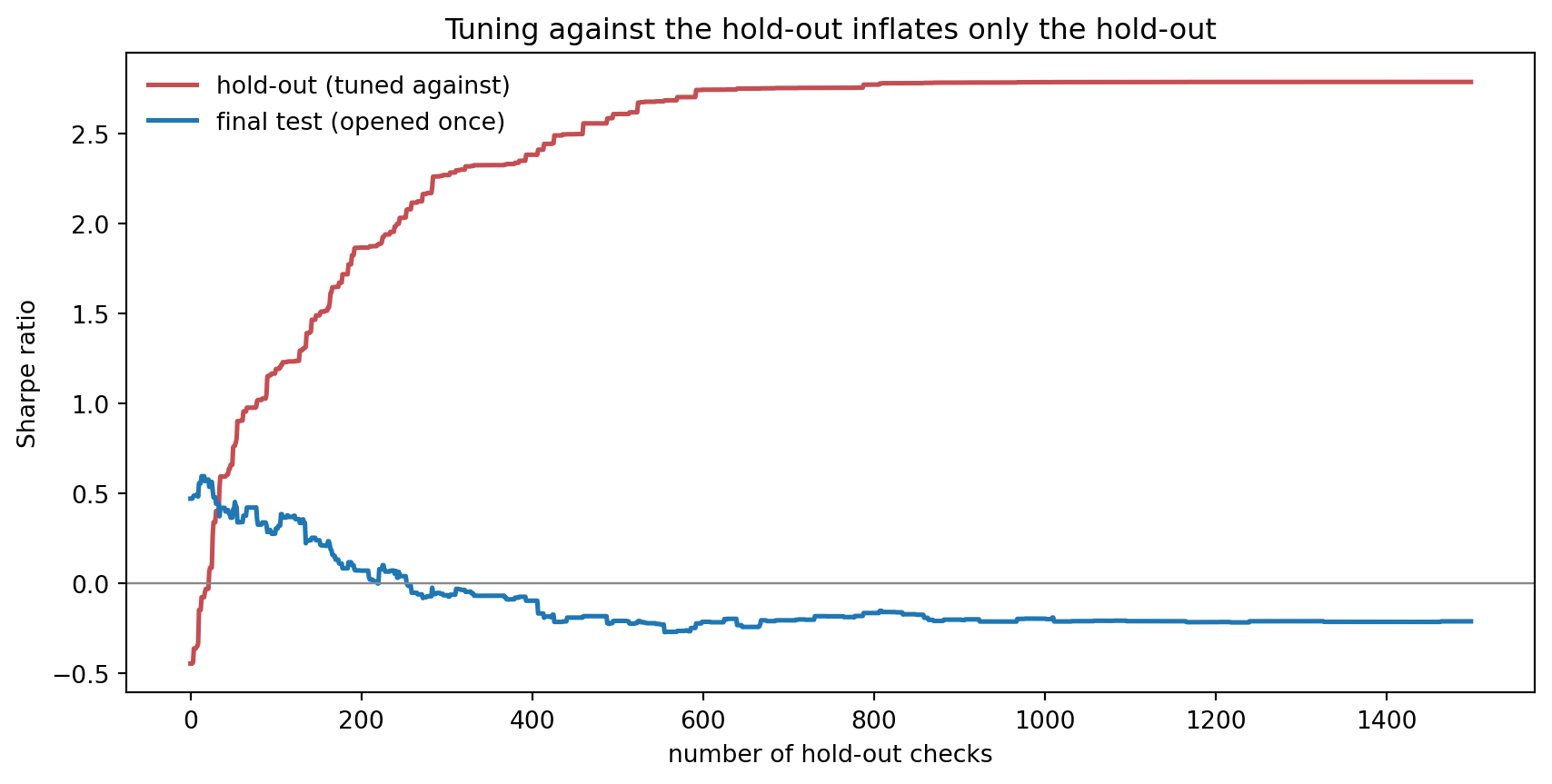

The red line is the hold-out Sharpe ratio, and it increases in small steps as I keep more changes. The teal line is the final test Sharpe ratio for the same strategy. The teal line does not follow the red line up, and it ends at −0.2.

The increase in the red line has a plain cause. In any three years of noise, some assets have a positive average return by luck and others a negative one. The loop keeps the weight changes that raise the hold-out Sharpe ratio, so round after round the strategy tends to buy assets that happened to do well in the hold-out and sell short assets that happened to do badly. The final test is drawn independently, so those weights have no expected edge there, and the same strategy has a Sharpe ratio close to zero on the final test.

Limitations

Tuning one strategy is not the same as testing many strategies at once. The best of many strategies has a high Sharpe ratio by chance alone, which I cover in an earlier post. Here there is one strategy, changed step by step after each look at the hold-out.

Real research uses the hold-out in more ways. My loop only changes weights, while in real research we also pick which years to include, which stocks to drop, and when to stop, each after seeing the last result. Every one of those choices is another look at the hold-out.

The numbers here are specific to this simulation. How much tuning inflates a real hold-out Sharpe ratio depends on the data, on how freely we search, and on how many times we check.

Conclusion

Decide in advance what result counts as a pass, then run the finished strategy on the final test once and accept the result. If it fails and we go back to research, those years are used up, and the next version needs a test that is still untouched. The cleanest such test is data that did not exist while we were working, which paper trading gives: the finished strategy runs forward on new days without real money. The takeaway is that a hold-out stops being out of sample the moment we optimise against it, because each choice made after seeing the hold-out fits the strategy to the hold-out’s noise.