About 5% of stocks created all the net wealth

Python

Analysis

Code

From 2000 to 2026, 5.4% of US stocks and 4.4% of European stocks created all the net wealth, the total gain above Treasury bills, repeating Bessembinder’s finding.

Published

April 24, 2026

Bessembinder (2018) found that the best-performing 4.3% of US stocks accounted for all of the net wealth the market created over Treasury bills, short-term US government debt, from 1926 to 2016. The remaining stocks, taken together, matched T-bills.

I test whether that concentration holds on modern data, for US and European stocks from 2000 to 2026. It does. The top 5.4% of US stocks account for 100% of net wealth created. In Europe the top 4.4% do the same.

The largest wealth creators are the mega-caps. Apple, Nvidia, Alphabet, and Microsoft lead the US list. Shell, HSBC, and BHP lead the European one. Slightly more than half of US stocks beat T-bills over their life in the sample, 5,611 of 10,061, or 55.8%. In Europe fewer than half did, 4,629 of 9,862, or 46.9%.

The method

Universe: US common stocks on NYSE and Nasdaq, and European stocks from 13 countries, 2000 to 2026, active and delisted. About 10,000 stocks in each region.
Wealth measure: Bessembinder’s Expression (3). Each month a stock creates or destroys wealth equal to its start-of-month market cap (share price times number of shares) times its excess return over T-bills (its return minus the T-bill return), compounded forward to the end of the sample at the T-bill rate.
I lag market cap to the previous month-end, so I know the capital at risk before the stock earns its return.
Risk-free rate: the one-month US T-bill from Kenneth French’s public data library, the source Bessembinder uses.
Concentration: sort stocks from highest to lowest wealth created, then read the cumulative share of the net total.

Starting point

The stock returns and market caps come from LSEG. Because the data is licensed, I cannot share the raw file, and I show the code without running it here. I print only aggregated totals. The one input I can show in full is the risk-free rate, which Kenneth French publishes for anyone to download.

Step 1. The risk-free rate

Bessembinder measures wealth against Treasury bills, so I need a monthly bill rate. Kenneth French publishes it in the same file as the Fama-French factors, as a zipped CSV file, a plain-text table, going back to 1926.

Code: the risk-free rate

import io                      # lets zipfile treat downloaded bytes as if they were a file
import zipfile                 # French publishes the factors as a zipped CSV
import urllib.request          # fetches the file over the web
import numpy as np
import pandas as pd

# Kenneth French's monthly one-month T-bill rate, the source Bessembinder uses.
url = "https://mba.tuck.dartmouth.edu/pages/faculty/ken.french/ftp/F-F_Research_Data_Factors_CSV.zip"

# urlopen hands back the file as bytes in memory, while zipfile expects something it can
# move around in, so BytesIO wraps those bytes to look like a file on disk.
downloaded_bytes = urllib.request.urlopen(url).read()
zip_in_memory = io.BytesIO(downloaded_bytes)
archive = zipfile.ZipFile(zip_in_memory)

# namelist() reports what is inside the archive. French's zip holds one CSV, so index 0 is it.
first_file_name = archive.namelist()[0]
csv_text = archive.read(first_file_name).decode("utf-8")

# ... parse the monthly block of csv_text out of the messy header and footer, into ff ...

ff["RF"] = ff["RF"] / 100                               # percent to decimal: 0.37 -> 0.0037

# The published file starts in 1926, and this study starts in 2000
ff_since_2000 = ff[ff["date"] >= "2000-01-01"]
rf_monthly = ff_since_2000.set_index("date")["RF"]

print(f"Monthly T-bill rates: {len(rf_monthly)} months")

# Read the ends after the count is printed. Indexing an empty series raises, and the
# count is the line that says the series is empty.
first_month = rf_monthly.index[0]
last_month = rf_monthly.index[-1]
mean_monthly_rf = rf_monthly.mean()

print(f"Period: {first_month.date()} to {last_month.date()}")
print(f"Mean monthly Rf: {mean_monthly_rf*100:.3f}% "
      f"(annualised: {mean_monthly_rf*12*100:.2f}%)")

Monthly T-bill rates: 314 months
Period: 2000-01-01 to 2026-02-01
Mean monthly Rf: 0.156% (annualised: 1.87%)

T-bills paid 1.9% a year over the period. The formula compounds each month’s excess wealth forward to the end of the sample at this rate, so I precompute a forward factor for every month: the remaining T-bill growth from that month to February 2026.

Code: the forward factor

# cumprod multiplies each month by the product of every month above it, so the months have to be in date order
# before it runs. The result is what one dollar left in T-bills is worth at each month end.
rf_in_date_order = rf_monthly.sort_index()
tbill_value = (1 + rf_in_date_order).cumprod()

# The last month is where every stock's wealth is measured, so the growth still to come
# after month t is the value at the end divided by the value at month t.
tbill_value_at_end = tbill_value.iloc[-1]
fv_forward = tbill_value_at_end / tbill_value           # remaining growth from month t to the end

print(f"Total T-bill compounding (2000-2026): {tbill_value_at_end:.3f}x")

Total T-bill compounding (2000-2026): 1.629x

A dollar left in T-bills grew to 1.6 times its size over the 26 years. The cumulative product used here is covered in Lesson 21 on the equity curve.

Step 2. Wealth created per stock

For each stock I walk its months in order and apply Bessembinder’s formula. Each month’s contribution is the lagged market cap times the excess return times the forward factor.

Code: the wealth created per stock

def compute_wealth(monthly_rows, rf_by_month, fv_by_month):
    """Bessembinder Expression (3): wealth = SUM_t mcap[t-1] * (ret[t] - rf[t]) * FV[t,T]."""
    # monthly_rows holds one stock's months in date order, each one a triple of the month,
    # that month's return, and the market cap at the month end. rf_by_month and fv_by_month
    # are the two series built in Step 1, and both are looked up by the month.
    wealth = 0.0
    mcap_last_month = np.nan                            # no lagged market cap before the loop runs

    for year_month, month_return, mcap_at_month_end in monthly_rows:
        # Nothing can be added until a lagged market cap exists, which rules out the first
        # month and any month before the stock's first reported cap.
        if not np.isnan(mcap_last_month):
            excess_return = month_return - rf_by_month[year_month]
            wealth += mcap_last_month * excess_return * fv_by_month[year_month]

        # Carry the month-end cap into the next month, where it is the capital at risk.
        # A month with no reported market cap keeps the previous month's market cap.
        if not np.isnan(mcap_at_month_end):
            mcap_last_month = mcap_at_month_end
    return wealth

I run this over every stock in each region. I read the daily returns in chunks, compound them to monthly gross returns, and take the market cap at each month-end. I cap daily returns at plus or minus 50% to remove erroneous prints.

The US totals:

Stocks: 10,061
Beat T-bills: 5,611 (55.8%)
Below T-bills: 4,450 (44.2%)
Net wealth created: $66,366,944M

The European totals:

Stocks: 9,862
Beat T-bills: 4,629 (46.9%)
Below T-bills: 5,233 (53.1%)
Net wealth created: $25,785,255M

US stocks created $66.4 trillion of net wealth above T-bills over the period. European stocks created $25.8 trillion.

Step 3. Concentration

I sort stocks from highest to lowest wealth created and read the cumulative share of the net total held by the top few percent.

Code: the concentration

def concentration(wealth_by_stock, pct_points):
    """Share of total net wealth created by the top X% of stocks."""
    ranked = wealth_by_stock.sort_values(ascending=False)   # biggest creators first
    net_wealth = ranked.sum()                               # winners minus losers
    n_stocks = len(ranked)

    shares = {}
    for pct in pct_points:
        # Round the count up, so the top 0.5% of 10,061 stocks is 51 stocks
        n_top = int(np.ceil(n_stocks * pct / 100))
        top_wealth = ranked.iloc[:n_top].sum()              # iloc slices by position
        shares[pct] = top_wealth / net_wealth * 100
    return shares


# The rows of the table below, from the top half percent to the top four percent
pct_points = [0.5, 1.0, 1.5, 2.0, 2.5, 3.0, 3.5, 4.0]

   Top %            US        Europe
    0.5%         60.7%         56.2%
    1.0%         72.2%         71.8%
    1.5%         79.4%         80.0%
    2.0%         84.8%         85.7%
    2.5%         88.6%         90.0%
    3.0%         91.5%         93.4%
    3.5%         94.0%         96.2%
    4.0%         96.0%         98.5%

The top 0.5% of US stocks created 60.7% of all the net wealth. The top 1.0% created 72.2%. At the top 4.0%, the share is 96.0%. The European share is below the US share at the top 0.5% and the top 1.0%, and above it from the top 1.5% onward. At the top 4.0% the European share is 98.5%.

The crossing point is the rank at which the cumulative share first equals 100%. I walk down the ranking until the running sum equals the net total, which gives it directly.

US: Top 541 stocks (5.4%) account for 100% of net wealth
Europe: Top 435 stocks (4.4%) account for 100% of net wealth

For the US that is the top 541 stocks, 5.4% of the 10,061 in the sample. For Europe it is the top 435 stocks, 4.4% of 9,862. So, the remaining 94.6% of US stocks and 95.6% of European stocks collectively matched Treasury bills over the 26 years.

Results

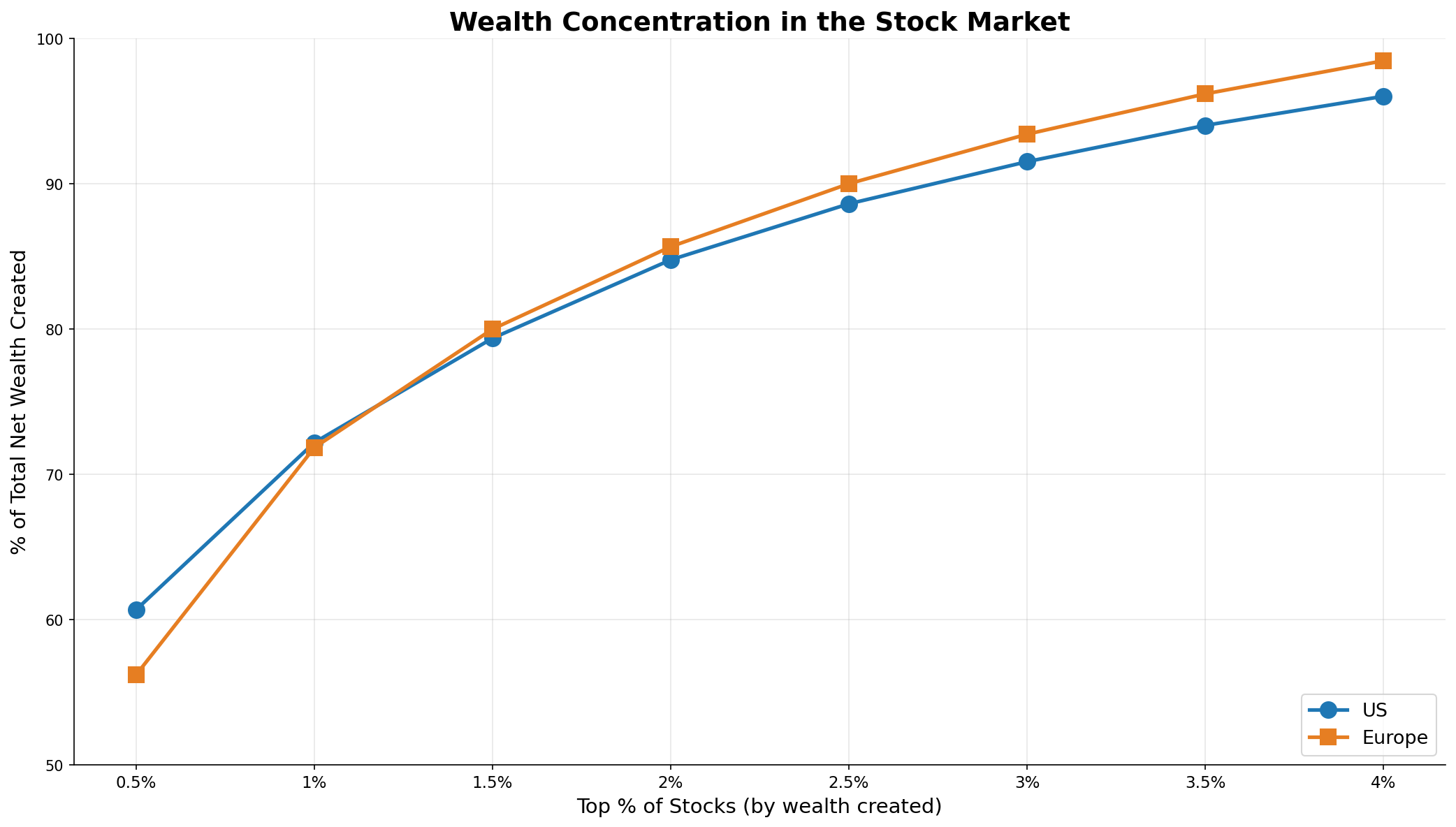
Cumulative share of net wealth created by the top few percent of stocks, US and Europe, 2000 to 2026.

In both regions the cumulative share increases steeply across the highest-ranked stocks and changes little after the top few percent. An even distribution would give a straight diagonal from the origin. The steeper the curve at the left, the larger the share of net wealth created by the highest-ranked stocks.

Limitations

One period, and a tech-heavy one. The rise of a small set of US mega-caps dominates 2000 to 2026. The concentration I measure partly reflects that regime, so a different quarter-century could place the crossing point elsewhere.

I measure invested capital with market cap. The formula weights each month by the previous month-end market cap, which treats the whole float as capital at risk. A large-cap stock changes the total more than a small-cap stock at the same excess return, so the largest companies are at both ends of the ranking.

I fill gaps in the risk-free series. Months with no French rate use 0.15% per month and months with no forward factor use 1.0. Few months need the fallback, so the effect on the totals is small.

I cap daily returns at plus or minus 50%. The cap removes erroneous prints. The cap also removes a handful of real extreme days, which lowers the wealth measured for the highest-ranked stocks.

Conclusion

The pattern Bessembinder found in the US from 1926 to 2016 shows up again on 2000-to-2026 data, in the US and in Europe. A few hundred stocks in each region account for all the net wealth created above Treasury bills, and the rest, as a group, earned the bill rate. Owning the broad market means we hold all of those few hundred stocks. The takeaway is that 541 US stocks and 435 European stocks created all the net wealth above T-bills between 2000 and 2026, so a portfolio that misses them earns close to the T-bill rate.