The Magic Formula worked. Just not lately.

Greenblatt’s Magic Formula returned 11.1% a year after trading costs, against 8.7% for the S&P 500 from 2001 to 2026, and has trailed it since about 2015.

Joel Greenblatt introduced the Magic Formula in The Little Book That Beats the Market. The formula is a mechanical rule that ranks stocks on two numbers. The first is earnings yield: earnings before interest and taxes (EBIT) divided by enterprise value, the market value of the company’s shares and debt minus its cash. The second is return on capital: EBIT divided by the capital the business employs. The rule buys the top of that ranking and holds each stock for a year. Greenblatt (2006) reports that it beat the market over his sample.

I test whether that held on US stocks from 2001 to 2026. Over the full 25 years it did. The Magic Formula returned 11.1% a year. The S&P 500 returned 8.7%. A dollar grew to 13.9 times its size. The same dollar in the index grew to 8.0 times.

The difference in return is concentrated in the first half of the sample. The Magic Formula returned more than the S&P 500 through about 2015 and less after that. Over the last five years the Magic Formula returned 6.6 percentage points a year less than the S&P 500. That is the pattern behind the Wall Street Journal piece on the formula that stopped working.

The strategy

• Universe: US common stocks, 2001 to 2026, active and delisted. I exclude financials and utilities, as Greenblatt prescribes, and keep the largest 3,500 stocks each month with a market cap (share price times number of shares) above $200m.
• Signal: rank each stock on earnings yield (EBIT over enterprise value) and on return on capital, then add the two ranks. A low combined score marks a stock with both a high earnings yield and a high return on capital.
• Portfolio: three new stocks a month from the top 30 by score, each month’s three held for twelve months as one tranche, so the portfolio, or book, holds about 36 stocks and turns over once a year. Equal weight.
• Costs: the bid-ask half-spread (half the gap between the price to buy and the price to sell) on each traded name plus a 0.05% commission.
• Benchmark: the S&P 500 total return, dividends reinvested.

I score on the ranks each month, because a single stock with a tiny enterprise value can have an earnings yield of several hundred percent and determine a level-based score on its own. Ranking each stock against the others each month keeps earnings yield and return on capital on the same scale.

Starting point

The backtest runs off one price-and-fundamentals file. Building it is a separate job that depends on the data vendor. I pull from LSEG Workspace. Because the data is licensed, the raw file stays off this page, and I show the code without running it here. The download route is the one from an earlier post, with the universe set to US common stocks and the fundamental fields added.

Step 1. The Magic Formula score

Each month I rank the eligible stocks on the two pieces and add the ranks.

NoteCode: the Magic Formula score

# One row of stock_months is one stock in one month.

# Earnings yield and return on capital, point-in-time (previous month's fundamentals).
stock_months["EY"] = stock_months["EBIT"] / stock_months["EV"]   # operating earnings over EV

# Keep only valid signals: positive EBIT, positive EV, positive return on capital.
# Each test gives a column of True and False, and & keeps the rows where all three hold.
# Naming them one at a time also avoids an operator-precedence error: in Python & binds tighter than >, so the
# three tests written on one line need a bracket around every comparison.
positive_ebit = stock_months["EBIT"] > 0
positive_ev = stock_months["EV"] > 0
positive_roc = stock_months["ROC"] > 0

# copy(): the rank columns added below belong to this table, and stock_months is left unchanged
eligible = stock_months[positive_ebit & positive_ev & positive_roc].copy()

# Cross-sectional ranks each month. Rank 1 in rank_EY has the highest earnings yield, and rank 1 in rank_ROC has the highest return on capital.
# groupby("month") ranks each stock against the others in the same month, which puts
# earnings yield and return on capital on one scale. method="first" settles a tie by row order,
# so two stocks never share a rank.
eligible["rank_EY"] = eligible.groupby("month")["EY"].rank(ascending=False, method="first")
eligible["rank_ROC"] = eligible.groupby("month")["ROC"].rank(ascending=False, method="first")

# The combined score. A stock with a low score has both a high earnings yield and a high return on capital.
eligible["score"] = eligible["rank_EY"] + eligible["rank_ROC"]

I cap the earnings yield at 50% and the return on capital at 200% before ranking. An earnings yield above 50% means EBIT is more than half of enterprise value, which I treat as stale trailing earnings after a large price decline.

Step 2. Greenblatt’s staggered book

Greenblatt staggers the rebalance, the regular change of holdings. Each month I buy the three best-scoring names not already held, and I sell each tranche twelve months later. At full capacity that is about 36 stocks, equal weighted, with one tranche rolling out and one rolling in each month. I charge costs only on the stocks that trade.

NoteCode: the staggered book

N_PER_TRANCHE = 3            # names bought each month
HOLD_MONTHS = 12             # months a tranche is held before it is sold

# tranches maps a buy month to the names bought in that month. Twelve of them are open once
# the book is full, and the dictionary holds the book from one month to the next.
tranches = {}
book_return_pieces = []      # one Series of daily book returns per month

for month in months:                                 # walk month by month
    # Sell the tranche that is now twelve months old. The second argument to pop() is what
    # to return when the key is absent, so the first twelve months sell an empty list.
    sold = tranches.pop(month - HOLD_MONTHS, [])

    # The names still in the book, collected from every tranche that is still open.
    held = set()
    for names in tranches.values():
        held.update(names)

    # Buy the three best-scoring names not already held.
    best_scoring = mf_screen[month]                  # top 30 by score this month
    not_held = [stock for stock in best_scoring if stock not in held]
    bought = not_held[:N_PER_TRANCHE]                # fewer than three if the screen is thin
    tranches[month] = bought

    # The book after this month's trade. The equal weight is spread over these names.
    book = held | set(bought)

    # Cost: half-spread plus commission on every name sold or bought this month.
    traded = set(sold) | set(bought)
    total_cost = sum(get_hs(stock, month) + COMMISSION for stock in traded)
    cost = total_cost / len(book)

    # Equal-weight daily return of the whole book. mean(axis=1) averages across the columns
    # of each row, so across the names held on that day.
    day_returns = daily.loc[daily["month"] == month, sorted(book)].mean(axis=1)

    # The month's cost is taken off each of that month's daily returns.
    book_return_pieces.append(day_returns - cost)

The staggering spreads the entry and exit dates across the year, so twelve rebalance dates contribute to the result instead of one. Each month the strategy trades only the tranche it sells and the three stocks it buys. Over the 25 years the average trading cost charged is about 0.4% a year.

The engine behind this is the one from Lesson 34 in Practical Coding, and Lesson 31 covers how the turnover is charged.

Step 3. Compare to the S&P 500

NoteCode: the performance measures

TRADING_DAYS = 252           # trading days in a year, for annualising


def performance(daily_returns):
    """Annualised return, annualised volatility, Sharpe ratio and cumulative growth."""
    # cumprod() multiplies the daily growth factors together, so nav is the value on each day
    # of one dollar invested at the start.
    nav = (1 + daily_returns).cumprod()
    final_value = nav.iloc[-1]                                # iloc[-1] is the last row

    years = len(daily_returns) / TRADING_DAYS
    annual_return = final_value ** (1 / years) - 1

    # Volatility scales with the square root of time when daily returns are independent
    annual_volatility = daily_returns.std() * np.sqrt(TRADING_DAYS)

    # No risk-free rate is subtracted, so this is return over volatility
    sharpe = annual_return / annual_volatility
    return annual_return, annual_volatility, sharpe, final_value

performance returns the annualised return, the annualised volatility (how much the returns swing), the Sharpe ratio (the return divided by the volatility) and the cumulative growth. The table below reports all of them except the volatility, and adds the worst drawdown, the largest fall from a previous peak.

                   Cumulative   Annualised   Sharpe   Max drawdown
S&P 500                  8.0x         8.7%     0.45         -54.7%
Magic Formula 30        13.9x        11.1%     0.44         -66.4%

Over the full sample the Magic Formula returned 11.1% a year against 8.7% for the S&P 500. The extra return came with more risk. The formula’s worst drawdown was 66.4%. The index’s was 54.7%. The two Sharpe ratios are almost identical at 0.44 and 0.45.

Results

Magic Formula portfolio against the S&P 500, 2001 to 2026. The top panel is cumulative return on a log scale. The bottom panel is the rolling five-year annualised premium, which is positive through 2015 and negative after that.

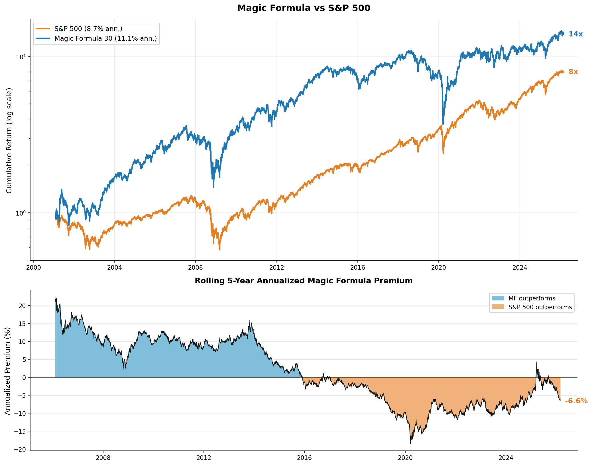
The bottom panel plots the rolling five-year premium of the Magic Formula over the S&P 500. It is positive, sometimes above 15 points a year, from the start through about 2015. So, the 2.4 percentage point difference in annual return comes from the first half of the sample. The rolling five-year premium has been negative since then, and it is minus 6.6 percentage points a year at the end of the sample.

Year by year, the Magic Formula returned more than the S&P 500 in 14 of the 26 calendar years the sample covers. The calendar-year difference is plus 25.7 percentage points in 2001 and plus 43.3 percentage points in 2009. It is minus 37.0 percentage points in 2019 and minus 19.6 percentage points in 2024.

Limitations

One specification. I ran a single version of the formula: EBIT over enterprise value, return on capital, top 30, monthly tranches. The thresholds and the portfolio size are choices, and I do not report results for other choices. I do not calculate a confidence interval, a range that likely contains the true value, for the difference in annual return.

Why the premium turned negative. I measure that the rolling five-year premium turned negative around 2015. I do not test why. This backtest does not separate the return of the Magic Formula ranking from the return of value stocks and smaller companies over the same years, and I do not test whether the premium turns positive again.

Costs are approximate. The half-spread and a flat commission understate the real cost of trading. Slippage past the quoted price is worse in smaller stocks, which the Magic Formula holds, so the true cost is higher than the 0.4% a year charged here.

Return on capital is a proxy. Greenblatt defines it on tangible capital employed. I use the closest field the vendor reports. I do not measure how far this ranking differs from a ranking on tangible capital employed.

Conclusion

The Magic Formula did beat the market over 25 years, with a mechanical rule that needs no forecasting. Then it stopped around 2015. Crowding after publication is one explanation for a premium that turns negative, and this backtest does not test it. The takeaway is that a strategy that returned more than the market over a long sample can stop doing so.

Read next

• The most profitable US companies beat the S&P 500, and the least profitable lost money The same quality-and-value idea, split into the best US stocks and the worst.
• Trading costs more than halved Swedish momentum’s ending value Another published strategy, and how much of its return remains after realistic trading costs.
• Do the highest-yielding stocks beat the S&P 500? Another rule that picks US stocks by one number, tested after trading costs.

Disclaimer: simplified, hypothetical backtest with approximate trading costs, for discussion purposes only. Not investment advice. Past performance does not guarantee future returns.

Data: US equity prices, fundamentals, and bid-ask quotes from LSEG Workspace (licensed). The S&P 500 total-return series is the benchmark. I do not reproduce the raw file here. Source: Joel Greenblatt, The Little Book That Beats the Market, 2006.