Which industries have won since 1926, and do winners stay winners?
In this post, I want to see which industries have been the long-term winners, who the current winner is, and what you can take from that for the future. Will the winners continue to be the winners?
I start by calculating what $1 in 1926 in each industry is worth today. I am looking at Kenneth French’s 12 industries, which are aggregated; otherwise, I would have 49 industries, each with its own niche, and the analysis could get less clear. Anyone more interested can take the code and do this analysis across the 49. The aggregation loses some information within these industries, because technology companies are grouped with other subindustries. The reason why I use these 12 is also that it is easy to get the data instead of computing it myself, and I do not have access to data as far back as Kenneth French has. I have attached the code in the appendix.
The winners in the long term
$1 in July 1926 is worth $60,367 in Business Equipment at the end of September 2026, and $59,679 in Healthcare, Medical Equipment, and Drugs. In the market, it is worth $19,567, and in Other, $2,244.
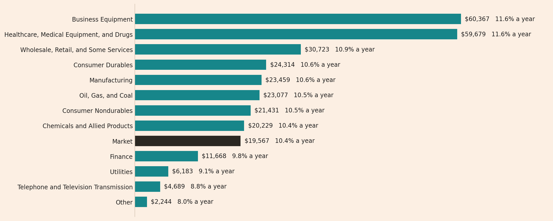
It is good to show explicitly what each of these industries means, as Kenneth French defines them.
| Industry | What it holds |
|---|---|
| Consumer Nondurables | Food, tobacco, textiles, apparel, leather, toys |
| Consumer Durables | Cars, TVs, furniture, household appliances |
| Manufacturing | Machinery, trucks, planes, office furniture, paper, commercial printing |
| Oil, Gas, and Coal | Coal mining, oil and gas extraction, petroleum refining |
| Chemicals and Allied Products | Industrial chemicals, plastics, soaps, cosmetics, paints, agricultural chemicals |
| Business Equipment | Computers, software, electronic equipment |
| Telephone and Television Transmission | Telephone, radio and television broadcasting, cable |
| Utilities | Electricity, natural gas, water supply |
| Wholesale, Retail, and Some Services | Wholesale, retail, laundries, repair shops |
| Healthcare, Medical Equipment, and Drugs | Health services, medical instruments, X-ray equipment, drugs |
| Finance | Banks, insurance, real estate, brokers, investment funds |
| Other | Mines, construction, building materials, transportation, hotels, business services, entertainment |
The current winner
Oil, Gas, and Coal is the current winner at the end of the sample period, which is September 2026. $1 at the end of 2025 is worth $1.42. That is not surprising, given where oil prices are, and it has performed much better than Business Equipment, at $1.22, which includes technology companies. But once again, Business Equipment also includes other types of companies that may not be technology companies.
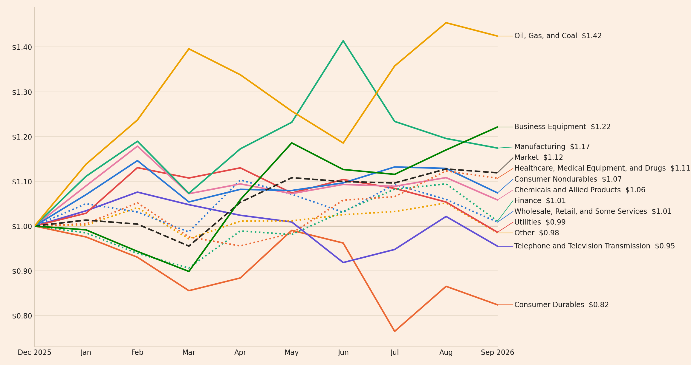
What you should take from here is who the current winner is and what the ranking of the other industries is, down to Consumer Durables at $0.82. With today’s news, it is easy to get fixated on technology companies and oil, but not the rest. So this is a way of seeing how the other industries have performed.
Does the winner stay the winner next year?
At the end of each year, I compute the cumulative 12-month return for each industry and rank them accordingly, where rank 1 is the highest return, rank 2 is the second-highest, and so forth. I do that for all the years. Then I go back to the first year with 12 months of data and ask: given the industry ranked 1st (the winner for that year), what will its ranking be the next year? If it ends up in the fourth position the next year, I count that as one in the fourth bar. Then I repeat that for the next year’s winner, and so on.
Mark Carhart makes this kind of table for mutual funds, and I adopt it for these industries. The formula is
\[\text{chance} = \frac{\begin{array}{c}\text{pairs of years in which the winner}\\ \text{has rank } r,\ h \text{ years later}\end{array}}{\text{all pairs of years, } h \text{ years apart}},\]
where \(r\) is the rank and \(h\) is the number of years later. In the animation below, \(h\) is 1, and \(r\) goes from 1 to 12.
The winner wins again next year in 17 of the 98 pairs of years, or 17.3%, and it is last in 13.
Does the winner stay the winner in later years?
Now I focus only on how often the winner in one year remains the winner the next year, and then I extend that to 2 years. So given the winner today, what is the proportion of times that it is the winner 2 years after, and then 3 years after, and then 4 years after? Each bar counts that exact year, whichever industry won in between. Carhart looks only at the next year, so this extension is mine.
Only the first bar, 1 year after the win, is above the dashed line. The dashed line puts all 98 possible bars together, from 1 year to 98 years after the win, where 528 of 4,851 pairs of years have the same winner, or 10.9%.
Does the winner so far stay the winner at the end of the year?
Once again, I do a ranking, but this time I compute the cumulative return for the first 3 months of the year and rank the industries. Then I count how often the winner (rank 1) after the 3-month return is still the winner at the end of the year, based on the 12-month return. I count it as one only when the winner is still the winner at the end of the year, and I repeat the process for all years. Then I do the same for 6 months and 9 months.
The winner after 3 months is still the winner at the end of the year in 36 of 99 years, after 6 months in 54, and after 9 months in 65. That is not surprising, because the first months are part of the whole year. Oil, Gas, and Coal is the winner after 9 months of 2026.
Limitations
The number of firms. A limitation is industry size, because the number of firms in each industry varies over time, and that can affect year-to-year performance. In July 1927, Telephone and Television Transmission held 5 firms.
No explanation. I compute these numbers without conditioning on anything else, so there can be other reasons why a winner continues to be a winner or the opposite, such as size. I am not claiming any causality. I am only showing some preliminary associations.
No statistical tests. I have not done any statistical testing, because this post is meant to be descriptive. So I cannot say whether the gap between 17.3% and 10.9% is more than chance.
The returns. All returns are before trading costs, in US dollars, and for US stocks.
Conclusion
In short, industries have performed differently over the years, and this year’s winner is not guaranteed to be next year’s winner. Only time will tell: as the year progresses and an industry remains the winner, its odds of winning at the end of the year increase, but that is not surprising.
Appendix: the code
import io
import urllib.request
import zipfile
from itertools import takewhile

import matplotlib.pyplot as plt
import pandas as pd

LIBRARY = "https://mba.tuck.dartmouth.edu/pages/faculty/ken.french/ftp/"
INDUSTRIES = {"NoDur": "Consumer Nondurables", "Durbl": "Consumer Durables",
              "Manuf": "Manufacturing", "Enrgy": "Oil, Gas, and Coal",
              "Chems": "Chemicals and Allied Products", "BusEq": "Business Equipment",
              "Telcm": "Telephone and Television Transmission", "Utils": "Utilities",
              "Shops": "Wholesale, Retail, and Some Services",
              "Hlth": "Healthcare, Medical Equipment, and Drugs", "Money": "Finance",
              "Other": "Other"}


def download(name):
    with urllib.request.urlopen(LIBRARY + name) as response:
        archive = zipfile.ZipFile(io.BytesIO(response.read()))
    return archive.read(archive.namelist()[0]).decode("latin-1")


def table_after(text, heading):
    lines = text.splitlines()
    first = next(number for number, line in enumerate(lines) if heading in line)
    start = next(number for number in range(first, len(lines)) if lines[number].startswith(","))
    rows = list(takewhile(str.strip, lines[start:]))
    table = pd.read_csv(io.StringIO("\n".join(rows)), index_col=0)
    table.columns = table.columns.str.strip()
    table.index = table.index.astype(str).str.strip()
    return table


text = download("12_Industry_Portfolios_CSV.zip")
monthly = table_after(text, "Average Value Weighted Returns -- Monthly").rename(columns=INDUSTRIES)
monthly.index = pd.PeriodIndex(monthly.index, freq="M")
annual = table_after(text, "Average Value Weighted Returns -- Annual").rename(columns=INDUSTRIES)
annual.index = annual.index.astype(int)
firms = table_after(text, "Number of Firms in Portfolios").rename(columns=INDUSTRIES)
factors = table_after(download("F-F_Research_Data_Factors_CSV.zip"), "Mkt-RF")
factors = factors[factors.index.str.len() == 6]
factors.index = pd.PeriodIndex(factors.index, freq="M")
market = factors["Mkt-RF"] + factors["RF"]
print(f"Months: {monthly.index[0]} to {monthly.index[-1]}, {len(monthly)}")
print(f"Calendar years: {annual.index[0]} to {annual.index[-1]}, {len(annual)}")
telephone = "Telephone and Television Transmission"
print(f"Firms in {telephone}, July 1927: {firms.at['192707', telephone]}")
Months: 1926-07 to 2026-09, 1203
Calendar years: 1927 to 2025, 99
Firms in Telephone and Television Transmission, July 1927: 5value = (1 + monthly / 100).prod()
value["Market"] = (1 + market.loc[monthly.index] / 100).prod()
value = value.sort_values(ascending=False)
a_year = 100 * (value ** (12 / len(monthly)) - 1)
print(pd.DataFrame({"$1 becomes": value.round(0), "% a year": a_year.round(1)}).to_string()) $1 becomes % a year
Business Equipment 60367.0 11.6
Healthcare, Medical Equipment, and Drugs 59679.0 11.6
Wholesale, Retail, and Some Services 30723.0 10.9
Consumer Durables 24314.0 10.6
Manufacturing 23459.0 10.6
Oil, Gas, and Coal 23077.0 10.5
Consumer Nondurables 21431.0 10.5
Chemicals and Allied Products 20229.0 10.4
Market 19567.0 10.4
Finance 11668.0 9.8
Utilities 6183.0 9.1
Telephone and Television Transmission 4689.0 8.8
Other 2244.0 8.0this_year = (1 + monthly.loc["2026-01":] / 100).cumprod()
this_year["Market"] = (1 + market.loc["2026-01":] / 100).cumprod()
print(this_year.iloc[-1].sort_values(ascending=False).round(2).to_string())
for months in [3, 6, 9]:
row = this_year.drop(columns="Market").iloc[months - 1]
print(f"Winner after {months} months: {row.idxmax()}, ${row.max():.2f}")Oil, Gas, and Coal 1.42
Business Equipment 1.22
Manufacturing 1.17
Market 1.12
Healthcare, Medical Equipment, and Drugs 1.11
Consumer Nondurables 1.07
Chemicals and Allied Products 1.06
Finance 1.01
Wholesale, Retail, and Some Services 1.01
Utilities 0.99
Other 0.98
Telephone and Television Transmission 0.95
Consumer Durables 0.82
Winner after 3 months: Oil, Gas, and Coal, $1.40
Winner after 6 months: Manufacturing, $1.41
Winner after 9 months: Oil, Gas, and Coal, $1.42winners = annual.idxmax(axis=1)
ranks = annual.rank(axis=1, ascending=False).astype(int)
next_rank = pd.Series([ranks.at[year + 1, winners[year]] for year in annual.index[:-1]])
print(next_rank.value_counts().sort_index().rename("years").to_string())1 17
2 6
3 5
4 6
5 10
6 6
7 1
8 6
9 15
10 8
11 5
12 13def same_winner(years_later):
same = winners.iloc[:-years_later].to_numpy() == winners.iloc[years_later:].to_numpy()
return same.sum(), same.size
distances = range(1, len(winners))
bars = pd.DataFrame([same_winner(distance) for distance in distances], index=distances,
columns=["same winner", "pairs of years"])
bars["chance, %"] = 100 * bars["same winner"] / bars["pairs of years"]
all_pairs = 100 * bars["same winner"].sum() / bars["pairs of years"].sum()
print(bars.head(5).round(1).to_string())
print(f"All {len(bars)} bars: {bars['same winner'].sum()} of {bars['pairs of years'].sum()}, "
f"{all_pairs:.1f}%") same winner pairs of years chance, %
1 17 98 17.3
2 6 97 6.2
3 10 96 10.4
4 9 95 9.5
5 8 94 8.5
All 98 bars: 528 of 4851, 10.9%growth = 1 + monthly.loc["1927-01":"2025-12"] / 100
rows = {}
for months in [3, 6, 9]:
first_months = growth[growth.index.month <= months]
so_far = first_months.groupby(first_months.index.year).prod()
still_winner = (so_far.idxmax(axis=1) == winners).sum()
rows[f"After {months} months"] = {"still the winner": still_winner, "of years": len(so_far),
"chance, %": round(100 * still_winner / len(so_far), 1)}
print(pd.DataFrame(rows).T.to_string()) still the winner of years chance, %
After 3 months 36.0 99.0 36.4
After 6 months 54.0 99.0 54.5
After 9 months 65.0 99.0 65.7BG, INK, GRID, SPINE = "#FCEFE3", "#1f1f1f", "#EADCCC", "#D5C6B4"
TEAL, DARK, RED = "#17868A", "#2b2822", "#C0392B"
PALE_RED, MUTED = "#e8b4a8", "#4a4a4a"
LINES = {"Consumer Nondurables": ("#2a78d6", "-"), "Consumer Durables": ("#eb6834", "-"),
"Manufacturing": ("#1baf7a", "-"), "Oil, Gas, and Coal": ("#eda100", "-"),
"Chemicals and Allied Products": ("#e87ba4", "-"), "Business Equipment": ("#008300", "-"),
"Telephone and Television Transmission": ("#6250d6", "-"), "Utilities": ("#e34948", "-"),
"Wholesale, Retail, and Some Services": ("#2a78d6", ":"),
"Healthcare, Medical Equipment, and Drugs": ("#eb6834", ":"), "Finance": ("#1baf7a", ":"),
"Other": ("#eda100", ":"), "Market": (DARK, "--")}
def style(figure, axis):
figure.patch.set_facecolor(BG)
axis.set_facecolor(BG)
axis.spines[["top", "right"]].set_visible(False)
axis.spines[["left", "bottom"]].set_color(SPINE)
axis.tick_params(axis="both", length=0, colors=INK)
ends = value.sort_values()
figure, axis = plt.subplots(figsize=(12.4, 6.4))
style(figure, axis)
axis.barh(ends.index, ends, color=[DARK if name == "Market" else TEAL for name in ends.index],
height=0.68)
for position, name in enumerate(ends.index):
axis.text(ends[name] + ends.max() * 0.012, position,
f"${ends[name]:,.0f} {a_year[name]:.1f}% a year", va="center", color=INK)
axis.set_xlim(0, ends.max() * 1.27)
axis.xaxis.set_visible(False)
axis.spines["bottom"].set_visible(False)
figure.savefig("industry_bars.png", dpi=170, bbox_inches="tight", facecolor=BG)
year_start = this_year.copy()
year_start.loc[pd.Period("2025-12", "M")] = 1.0
year_start = year_start.sort_index()
final = year_start.iloc[-1].sort_values()
places = final.tolist()
for number in range(1, len(places)):
places[number] = max(places[number], places[number - 1] + 0.024)
positions = range(len(year_start))
figure, axis = plt.subplots(figsize=(13.6, 7.2))
style(figure, axis)
axis.axhline(1, color=SPINE, lw=1.4)
for name, place in zip(final.index, places):
color, line_style = LINES[name]
axis.plot(positions, year_start[name], color=color, ls=line_style, lw=2.2)
axis.plot([positions[-1], positions[-1] + 0.3], [final[name], place],
color=color, lw=0.9, clip_on=False)
axis.text(positions[-1] + 0.33, place, f"{name} ${final[name]:.2f}",
va="center", color=INK, clip_on=False)
axis.set_xlim(0, positions[-1])
axis.set_xticks(list(positions),
["Dec 2025", "Jan", "Feb", "Mar", "Apr", "May", "Jun", "Jul", "Aug", "Sep 2026"])
axis.yaxis.set_major_formatter(lambda number, _: f"${number:.2f}")
axis.grid(True, axis="y", color=GRID)
figure.subplots_adjust(left=0.05, right=0.72, top=0.98, bottom=0.05)
figure.savefig("industry_2026.png", dpi=170, facecolor=BG)
first_five = bars.head(5)
figure, axis = plt.subplots(figsize=(10, 6))
style(figure, axis)
axis.bar(first_five.index, first_five["chance, %"], width=0.42, color=PALE_RED, zorder=2)
axis.plot(first_five.index, first_five["chance, %"], marker="o", lw=2.6, ms=9, color=RED, zorder=3)
axis.axhline(all_pairs, color=MUTED, lw=1.2, ls="--", zorder=4)
axis.text(5.75, all_pairs + 0.3, f"{all_pairs:.1f}% of all pairs of years have the same winner",
color=MUTED, ha="right", va="bottom")
for distance, row in first_five.iterrows():
label = f"{row['chance, %']:.1f}%\n{row['same winner']:.0f} of {row['pairs of years']:.0f}"
axis.annotate(label, (distance, row["chance, %"]), textcoords="offset points",
xytext=(-16, 11) if distance == 1 else (32, -30), color=INK)
axis.set_xlabel("Years after the win", color=MUTED)
axis.set_ylabel("Chance that the same industry is the winner", color=MUTED)
axis.set_ylim(0, 24)
axis.set_xlim(0.6, 5.8)
axis.set_xticks(first_five.index)
axis.yaxis.set_major_formatter(lambda number, _: f"{number:.0f}%")
axis.grid(True, axis="y", color=GRID)
axis.set_axisbelow(True)
figure.savefig("industry_winner.png", dpi=150, bbox_inches="tight", facecolor=BG)Read next
- How to use Kenneth French’s data library
- Who wins in size and momentum?
- Using the Fama-French factors in Python to test a portfolio’s alpha
Disclaimer: a teaching example, not investment advice.
Data and sources: Kenneth R. French, Data Library, 12 Industry Portfolios, its industry definitions, and Fama/French 3 Factors, downloaded on 3 November 2026 (built from the Center for Research in Security Prices (CRSP) database of September 2026). Mark M. Carhart, “On Persistence in Mutual Fund Performance”, Journal of Finance (1997).