How to use Kenneth French’s data library
I wrote this post as an easy-to-follow guide to using Kenneth French’s data. It is a rich data library that you can use both to map out the different factors’ performance and to test whether a strategy you have found is due to any of these factor exposures or to something they cannot explain, in the sense that your strategy has an alpha if the intercept is positive and statistically significant.
Step 1. Sorting the stocks
- A New York Stock Exchange (NYSE) stock
- An American Stock Exchange (AMEX) or National Association of Securities Dealers Automated Quotations (NASDAQ) stock
- A larger dot is a larger stock
Normally, the grouping is based on the one characteristic that you want to form a factor on, here book-to-market. But size is often used as an additional sorting variable to avoid the well-known confounding, in the sense that differences in book-to-market could be just due to size differences. That is why size is included, even though the interest is in the value factor.
The cutoffs come from NYSE stocks because those are on average the biggest firms. If an exchange with much smaller stocks set the cutoff, it would misrepresent what a big company truly is. The opposite is less likely, since when big companies set the cutoff, the stocks they define as small are still small.
The returns are value-weighted because small stocks should not drive them, which could happen with equal weights. Small stocks are also more prone to trading costs, which would make the returns less realistic, because the gap between gross and net returns would be larger.
Step 2. Building the factors
This table shows how the factors are constructed and how the returns of those factors are computed. They share sorting on size, which is well known to be a confounder, or could be one. For example, the differences between value stocks and growth stocks may be more due to size differences. That is why size is also a sorting variable for the other factors, and for the size factor itself, book-to-market is the second sorting variable. The factors differ by the variable that is of interest to compute as a factor, and momentum is also sorted every month.
| Factor | Sorted on | How the variable is measured | When | Return each month |
|---|---|---|---|---|
| Small minus big (SMB) | Size and book-to-market | Market cap at the end of June | Every June | Average of the three small groups − average of the three big groups |
| High minus low (HML) | Book-to-market and size | Book equity for the fiscal year ending in t − 1 ÷ market cap at the end of December of t − 1 | Every June of year t | ½ × (small value − small growth) + ½ × (big value − big growth) |
| Robust minus weak (RMW) | Operating profitability and size | (Revenue − cost of goods sold − selling, general and administrative costs − interest expense) ÷ (book equity + minority interest), fiscal year ending in t − 1 | Every June of year t | ½ × (small robust − small weak) + ½ × (big robust − big weak) |
| Conservative minus aggressive (CMA) | Investment and size | Change in total assets from the fiscal year ending in t − 2 to the one ending in t − 1 ÷ total assets at t − 2 | Every June of year t | ½ × (small conservative − small aggressive) + ½ × (big conservative − big aggressive) |
| Momentum (Mom) | Past return and size | Return from 12 months to 2 months before | Every month | ½ × (small winners − small losers) + ½ × (big winners − big losers) |
| Short-term reversal (ST_Rev) | Last month’s return and size | Return over the last month | Every month | ½ × (small losers − small winners) + ½ × (big losers − big winners) |
| Long-term reversal (LT_Rev) | Past return and size | Return from 60 months to 13 months before | Every month | ½ × (small losers − small winners) + ½ × (big losers − big winners) |
Size is the market cap at the end of June, and for the three factors sorted monthly, at the end of the previous month. In the US factor files, every size split is at the NYSE median, and every split on the other variable is at the NYSE 30th and 70th percentiles. In the five-factor file, SMB averages the size spreads from the book-to-market, profitability, and investment sorts.
Step 3. Reading the other files
Every time you open a portfolio file, you get some time series of returns that can be either value-weighted or equal-weighted, monthly or annual (daily returns are in separate files), so you really need to pay attention to what the headings say. Then look at the number of firms and the average market cap in the sorted groups, as well as the value-weighted average of the sorting variable, such as book-to-market. And you should pay attention when you see a return of −99.99 or −999, because that indicates a missing return rather than a return in itself.
| Variable | How it is measured | Sorted |
|---|---|---|
| Earnings to price (E/P) | Earnings before extraordinary items for the fiscal year ending in t − 1 ÷ market cap at the end of December of t − 1 | Every June of year t |
| Cash flow to price (CF/P) | (Earnings before extraordinary items + equity’s share of depreciation + deferred taxes) for the fiscal year ending in t − 1 ÷ market cap at the end of December of t − 1 | Every June of year t |
| Dividend yield (D/P) | Dividends paid from July of t − 1 to June of t ÷ market cap in June of t | Every June of year t |
| Market beta | From the past 60 months of returns (24 at least) | Every June |
| Accruals | Change in operating working capital per split-adjusted share from fiscal year-end t − 2 to t − 1 ÷ book equity per share in t − 1 | Every June of year t |
| Net share issues | Change in the log of split-adjusted shares outstanding from fiscal year-end t − 2 to t − 1 | Every June of year t |
| Variance | Variance of daily returns over the past 60 trading days (20 at least) | Every month |
| Residual variance | The same, for what the three-factor model leaves unexplained | Every month |
| Past returns | Months 12 to 2 before (momentum), last month (short-term reversal), months 60 to 13 before (long-term reversal) | Every month |
In the US files, stocks are sorted based on cutoff values, or percentiles, derived from NYSE stocks only. And Kenneth French also publishes these cutoffs, for example, the market cap cutoffs of NYSE stocks each month.
Step 4. Using the international files
The international files contain the same methodology that is already covered, but applied to other data sets than US stocks, such as Europe. The main difference is that the split is not based on the NYSE, but on the region’s market cap (for emerging markets, each country’s). Big stocks are the largest ones that together make up 90% of the region’s market cap,
\[\text{stock } i \text{ is big if } \sum_{j=1}^{i} \text{market cap}_j \le 0.9 \sum_{j=1}^{N} \text{market cap}_j,\]
where the stocks are ranked by their market cap at the end of June (for momentum, at the end of every month), from the largest, \(j = 1\), to the smallest, \(j = N\). The cutoffs on book-to-market and the other variables come from these big stocks only.
| Files | Size cutoffs | Cutoffs on the other variable |
|---|---|---|
| Factors and 2 × 3 groups | Big: the largest stocks that together make up 90% of the market cap | 30th and 70th percentiles of the big stocks |
| 25 groups (5 × 5) | 3%, 7%, 13%, and 25% of the market cap, counted from the smallest stock | 20th, 40th, 60th, and 80th percentiles of the big stocks |
| Developed and Developed ex US | From all the stocks of the combined region | From each of its regions separately |
| Emerging markets | From each country | From each country |
| Momentum files | As above, but sorted at the end of every month | As above, on the return from 12 months to 2 months before |
| Country value and growth files | No size split | Top and bottom 30% of each country’s stocks, sorted every December |
The market factor is the region’s value-weighted market return minus the US Treasury bill, because all the returns are quoted in dollars. So you have a dollar exposure in the return. To remove it, for example, to measure a Swedish portfolio against the European files (since there are no Swedish factor files), you need to convert the returns from dollars to kronor.
\[ \begin{aligned} \text{group or market return: } & R_{\text{SEK}} = (1 + R_{\text{USD}})(1 + x) - 1\\ \text{long-short factor: } & F_{\text{SEK}} = (1 + x)\, F_{\text{USD}}\\ \text{market factor: } & R^{\text{market}}_{\text{SEK}} - \text{RF}_{\text{SEK}}\\[4pt] \text{so: } & \text{the currency enters the group}\\ & \text{and market returns in full}\\ & \text{and mostly cancels}\\ & \text{in a long-short factor}\\[4pt] \text{with: } & \text{SEK} = \text{Swedish kronor}\\ & \text{USD} = \text{US dollars}\\ & x = \text{the month's change in the krona}\\ & \quad \text{price of a dollar}\\ & R^{\text{market}}_{\text{USD}} = (\text{Mkt} - \text{RF}) + \text{RF}\\ & \text{RF}_{\text{SEK}} = \text{a Swedish risk-free rate,}\\ & \quad \text{all returns as decimals} \end{aligned} \]
Step 5. Checking the recipe
Here I use the values in the data files to compute the factors, then check them against what is published as a robustness check. They all match, up to the rounding in his files. The chart shows the rebuilt HML against his published HML, one dot per month, and every dot lies on the diagonal.
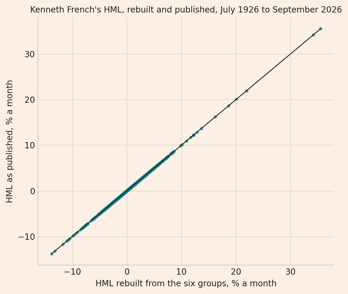
1203 months, 1926-07 to 2026-09
Largest difference, percentage points:
HML    0.005
SMB    0.005
Conclusion
In this post, I show how to use Kenneth French’s data files and how he computes the factors himself.
Appendix: the code
import io
import urllib.request
import zipfile
from itertools import takewhile

import matplotlib.pyplot as plt
import pandas as pd

LIBRARY = "https://mba.tuck.dartmouth.edu/pages/faculty/ken.french/ftp/"


def download(name):
    with urllib.request.urlopen(LIBRARY + name) as response:
        archive = zipfile.ZipFile(io.BytesIO(response.read()))
    return archive.read(archive.namelist()[0]).decode("latin-1")


def monthly_table(text):
    lines = text.splitlines()
    start = next(number for number, line in enumerate(lines) if line.startswith(","))
    rows = list(takewhile(str.strip, lines[start:]))
    table = pd.read_csv(io.StringIO("\n".join(rows)), index_col=0)
    table.index = pd.PeriodIndex(table.index.astype(str), freq="M")
    return table.replace([-99.99, -999], float("nan"))


six = monthly_table(download("6_Portfolios_2x3_CSV.zip"))
factors = monthly_table(download("F-F_Research_Data_Factors_CSV.zip"))

small_growth = six["SMALL LoBM"]
small_middle = six["ME1 BM2"]
small_value = six["SMALL HiBM"]
big_growth = six["BIG LoBM"]
big_middle = six["ME2 BM2"]
big_value = six["BIG HiBM"]
hml = (small_value + big_value) / 2 - (small_growth + big_growth) / 2
smb = (small_growth + small_middle + small_value) / 3 - (big_growth + big_middle + big_value) / 3

months = six.index.intersection(factors.index)
difference = pd.DataFrame({"HML": hml[months] - factors.loc[months, "HML"],
                           "SMB": smb[months] - factors.loc[months, "SMB"]})
print(f"{len(months)} months, {months[0]} to {months[-1]}")
print("Largest difference, percentage points:")
print(difference.abs().max().round(3).to_string())

BG, INK, GRID, SPINE, TEAL = "#FCEFE3", "#1f1f1f", "#EADCCC", "#D5C6B4", "#17868A"
fig, axis = plt.subplots(figsize=(6.4, 5.4))
axis.scatter(hml[months], factors.loc[months, "HML"], s=9, color=TEAL, alpha=0.6)
ends = [hml[months].min(), hml[months].max()]
axis.plot(ends, ends, color=INK, lw=1)
axis.set_xlabel("HML rebuilt from the six groups, % a month", color=INK)
axis.set_ylabel("HML as published, % a month", color=INK)
axis.set_title("Kenneth French's HML, rebuilt and published, July 1926 to September 2026",
               color=INK, fontsize=10)
fig.patch.set_facecolor(BG)
axis.set_facecolor(BG)
axis.grid(True, color=GRID, lw=1.0)
axis.set_axisbelow(True)
axis.spines[["top", "right"]].set_visible(False)
axis.spines[["left", "bottom"]].set_color(SPINE)
axis.tick_params(axis="both", length=0, colors=INK)
fig.savefig("french_hml_check.png", dpi=200, bbox_inches="tight")
Read next
- Using the Fama-French factors in Python to test a portfolio’s alpha How to download the factors and test whether a portfolio has an alpha.
- Testing a stock characteristic as a factor How the factors explain the returns of French’s 25 groups, and how to test whether a strategy has an alpha.
- How to do factor investing Value and momentum in a long-only portfolio, with rebalancing and trading costs.
Disclaimer: an explanation of public data files, for teaching. Not investment advice.
Data and sources: Kenneth R. French, Data Library, its files and their description pages, downloaded on 29 October 2026 (built from the CRSP database of September 2026). Eugene F. Fama and Kenneth R. French, “Common risk factors in the returns on stocks and bonds”, Journal of Financial Economics (1993), and “A five-factor asset pricing model”, Journal of Financial Economics (2015). James L. Davis, Eugene F. Fama and Kenneth R. French, “Characteristics, covariances, and average returns: 1929 to 1997”, Journal of Finance (2000), for book equity.