Asset allocation for every economic environment
In 2008, US stocks lost 37% after inflation, and US Treasuries gained 20%. In 2022, stocks lost 25%, and Treasuries lost 21%. In 2008, the economy shrank and inflation decreased to almost zero. In 2022, inflation was far above what investors had expected.
Asset allocation is the choice of how much of a portfolio to put in each asset class, such as stocks, government bonds, gold and commodities. From 1971 to 2025, each of these four asset classes earned a positive average return after inflation, yet each also stayed below an earlier high for at least 13 years. After inflation, US stocks, for example, were worth less at the end of every year from 2000 to 2012 than at the end of 1999.
An asset manager starts from the investor’s required return, risk tolerance and time horizon. These set how much risk the portfolio can take. To spread that risk, the manager asks three questions:
- In which economic environments does each asset class gain, and in which does it lose?
- How volatile is each asset class, and how correlated are the asset classes?
- How much of the portfolio’s risk comes from each asset class?
The answers let the manager set each asset class’s weight so that the portfolio does not depend on any one environment.
Growth and inflation define four environments
Bridgewater Associates defines four economic environments by two surprises (Bridgewater, 2012). Growth can be above or below what investors expected, and so can inflation. Prices already reflect expectations, so the surprise is what moves them. A year can be in two environments at once, as 1974 was, with growth below expectations and inflation above. The picture shows which of the four asset classes tend to gain in each environment.
Bridgewater’s All Weather portfolio, built on this idea, gives each of the four environments the same share of its risk.
Different asset classes gained in 1974, 2008 and 2022
Gold and commodities gained after inflation in 1974, Treasuries and gold in 2008, and commodities in 2022. The chart gives each asset class’s calendar-year return after inflation and that of a 60/40 portfolio. That portfolio holds 60% in US stocks and 40% in US Treasuries, rebalanced annually. I take inflation out of each return with
\[\text{return after inflation} = \frac{1 + \text{return}}{1 + \text{inflation}} - 1,\]
where inflation is the change in US consumer prices over the same twelve months. If $1 grows to $1.10 while prices rise 5%, for example, the return after inflation is 1.10 / 1.05 − 1 = 4.8%.
The 60/40 portfolio lost in all three years. In 1974 and 2022, inflation was above expectations, and the 60/40 portfolio holds neither gold nor commodities, the asset classes that tend to gain then. In 2008, its stocks lost 37% and its Treasuries gained 20%, so it lost 0.6 × 37% − 0.4 × 20% = 14%.
87% of a 60/40 portfolio’s risk came from stocks
Most of the 60/40 portfolio’s risk came from its stocks, which had a 60% weight and were about twice as volatile as Treasuries. From February 1970 to December 2025, the annualized volatility of monthly returns was 16% for US stocks, 8% for US Treasuries, 19% for gold and 20% for commodities.
The correlation between stocks and Treasuries depends on the environment. An earlier post finds a correlation of −0.31 on monthly returns over 2008 to 2013, after the financial crisis, and +0.53 over 2021 to 2026, years that included the inflation of 2022. So Treasuries tend to offset stocks when growth is below expectations, and to fall with them when inflation is above (Lombardi and Sushko, 2023).
An asset class’s share of risk is the part of the portfolio’s variance that comes from that asset class:
\[\text{share of risk} = \frac{\text{weight} \times \text{covariance}}{\text{variance of the portfolio}},\]
where the covariance is between the asset class’s return and the portfolio’s return. The covariance is larger when the asset class is more volatile and more correlated with the portfolio. The shares of risk of all the asset classes add up to 100%. An equal-risk portfolio, also called a risk-parity portfolio, sets its weights so that each asset class has the same share of risk. The chart compares the two portfolios, with the volatilities and correlations of 1970 to 2025.
So from 1970 to 2025, the 60/40 portfolio split its money 60/40 and its risk 87/13. In traditional portfolios, more than 80% of the risk comes from stocks (Pedersen, 2015).
The equal-risk portfolio puts 45% in Treasuries, the least volatile asset class, and 17% to 21% in each of the other three. It gives each asset class the same share of risk, while All Weather aims to give each environment the same share. The two rules differ because commodities and gold both tend to gain when inflation is above expectations, while only Treasuries tend to gain when growth is below. So equal risk for each asset class means twice as much risk in gold and commodities as in Treasuries.
The equal-risk portfolio earned less and lost less
The equal-risk portfolio paid for smaller losses with a lower return. In 1974, 2008 and 2022, it returned 1%, −5% and −13% after inflation. The 60/40 portfolio returned −24%, −14% and −23%.
The chart follows $1 in each portfolio from the end of 1970 to the end of 2025, after inflation. Both portfolios are hypothetical and rebalanced annually, and the equal-risk weights use the volatilities and correlations of the whole period.
The 60/40 portfolio was worth less at the end of every year from 1973 to 1982 than at the end of 1972, ten years in a row. The equal-risk portfolio’s longest such run was four years, from 2013 to 2016.
After inflation, $1 grew to $21 in the 60/40 portfolio, or 5.6% a year. In the equal-risk portfolio, it grew to $14, or 4.9% a year. Treasuries, which make up 45% of the equal-risk portfolio, returned 2.4% a year after inflation. Bridgewater’s All Weather portfolio uses leverage to aim for a higher return with the same balance of risk. Leverage adds the risk of forced selling at a loss.
Limitations
The equal-risk weights use risk measured after the fact. No manager knew in 1971 the volatilities and correlations of 1970 to 2025, and they change over time. So the chart shows how the rule works, with weights chosen in hindsight.
The environments describe what an asset class tends to do. Gold lost 6% after inflation in 2022, a year of high inflation. Erb and Harvey (2013) find that gold is an unreliable hedge against inflation over practical investment horizons.
The portfolios hold four US asset classes, before costs and taxes. The Treasury return is computed from the 10-year yield, gold’s from its spot price, and the commodities’ from the S&P GSCI Total Return index.
Conclusion
The takeaway is that an asset manager spreads a portfolio’s risk across environments, within the investor’s risk tolerance. Equal shares of risk are one rule, and a manager can give one environment more risk on purpose when the investor’s needs call for it.
Appendix: the code
The notebook reads the files that the notebook of the correlation post saves, and it downloads US consumer prices from FRED once. I show the code without running it here, with the output of my run.
from pathlib import Path
import json

import matplotlib.pyplot as plt
import matplotlib.ticker as mticker
import numpy as np
import pandas as pd
import requests
from scipy.optimize import minimize

# The notebook of the post on correlations with US stocks saved three files in the home folder.
# Path.home() is that folder, and / joins a folder and a file name
STOCK_FILE = Path.home() / "us_stock_daily.csv"                  # US stocks, from Kenneth French
TREASURY_YIELD_FILE = Path.home() / "treasury_yield_daily.csv"   # the 10-year yield, from FRED
LSEG_FILE = Path.home() / "lseg_levels_daily.csv"                # gold and commodities, from LSEG
# This notebook downloads US consumer prices from FRED once and saves them in the home folder too
CONSUMER_PRICES_FILE = Path.home() / "us_consumer_prices_monthly.csv"
CONSUMER_PRICES_URL = "https://fred.stlouisfed.org/graph/fredgraph.csv?id=CPIAUCNS"
# Path.cwd() is the folder this notebook runs in
NUMBERS_FILE = Path.cwd() / "asset_allocation_numbers.json"      # the numbers the charts draw
CHART_FILE = Path.cwd() / "asset_allocation.png"

BOND_MATURITY = 10                               # the rebuilt Treasury is a 10-year bond
GOLD_SCALE_BREAK = pd.Timestamp("1989-10-16")    # the first day LSEG quotes the whole gold price
FIRST_YEAR, LAST_YEAR = 1971, 2025               # the years with returns for all four asset classes
FIRST_MONTH, LAST_MONTH = "1970-02", "2025-12"   # the months behind the volatilities
YEARS = [1974, 2008, 2022]                       # the three years the post compares
STOCK_SHARE = 0.6                                # the 60/40 portfolio's share of money in stocks
ASSETS = ["stocks", "treasury", "gold", "commodities"]
PORTFOLIOS = ["60/40", "equal risk"]
# The names in the printed tables and on the chart
NAMES = {"stocks": "US stocks", "treasury": "US Treasuries", "gold": "Gold",
         "commodities": "Commodities", "60/40": "60/40 portfolio",
         "equal risk": "Equal-risk portfolio", "inflation": "Inflation"}

# The site's chart colours, in this order: the cream background, the text, the light grid lines,
# the pale frame and the axis labels. RED and TEAL are the two portfolios' lines
BG, INK, GRID, SPINE, AXIS_TEXT = "#FCEFE3", "#1f1f1f", "#EADCCC", "#D5C6B4", "#4a4a4a"
RED, TEAL = "#C0392B", "#17868A"def bond_price(bond_yield, coupon_rate, years_left):
"""The price, per 100 of face value, of a bond that pays its coupon twice a year.
bond_price(0.05, 0.05, 10) is 100, because a bond whose coupon rate equals its yield is worth
its face value."""
# ** raises to a power, so discount is the value today of 1 paid when the bond matures
discount = (1 + bond_yield / 2) ** (-2 * years_left)
return 100 * (coupon_rate / bond_yield * (1 - discount) + discount)
def treasury_return(bond_yield):
"""Each day's return on a Treasury that stays a 10-year bond, rebuilt from its yield as in the
correlation post. Each day, a 10-year bond bought the day before at 100, with a coupon rate
equal to that day's yield, is priced at the new yield. Its return is the change in its price
plus the coupon earned over the days in between."""
# diff() gives the days since the row before, which is more than 1 after a weekend, and
# clip(lower=1) counts a repeated date as 1 day
years_passed = bond_yield.index.to_series().diff().dt.days.clip(lower=1) / 365
yield_before = bond_yield.shift(1) # shift(1) moves each yield one row down
new_price = bond_price(bond_yield, yield_before, BOND_MATURITY - years_passed)
daily_return = (new_price - 100) / 100 + yield_before * years_passed
return daily_return.dropna() # the first day has no day before it
# read_csv reads a file into a table. parse_dates reads the Date column as dates, and set_index
# makes the dates the row labels
stocks = pd.read_csv(STOCK_FILE, parse_dates=["Date"]).set_index("Date")["level"]
treasury_yield = pd.read_csv(TREASURY_YIELD_FILE, parse_dates=["Date"]).set_index("Date")["yield"]
lseg = pd.read_csv(LSEG_FILE, parse_dates=["Date"]).set_index("Date").sort_index()
# DataFrame.loc[rows, column] selects rows and a column. LSEG quotes half the gold price before
# GOLD_SCALE_BREAK, so *= 2 doubles those prices and gives the series one scale
lseg.loc[lseg.index < GOLD_SCALE_BREAK, "gold"] *= 2
# The yields are percentages, so / 100 makes them fractions. cumprod() multiplies the daily growth
# factors, 1 + return, into a level
treasury = (1 + treasury_return(treasury_yield / 100)).cumprod()
# concat puts the four series side by side, matched by date, with the keys as column names
levels = pd.concat({"stocks": stocks, "treasury": treasury, "gold": lseg["gold"],
"commodities": lseg["commodities"]}, axis=1).sort_index()
for asset in ASSETS:
days_with_level = levels[asset].dropna() # dropna() leaves out the days without a level
# {x:,} writes commas between thousands, {date:%d %b %Y} a date such as 02 Jan 1970, and
# {text:<14} pads the text to 14 characters
print(f"{NAMES[asset]:<14} {len(days_with_level):,} days, "
f"{days_with_level.index[0]:%d %b %Y} to {days_with_level.index[-1]:%d %b %Y}")US stocks 26,296 days, 01 Jul 1926 to 31 Jul 2026
US Treasuries 16,160 days, 03 Jan 1962 to 15 Sep 2026
Gold 14,747 days, 22 Mar 1968 to 17 Sep 2026
Commodities 14,296 days, 02 Jan 1970 to 17 Sep 2026# One level a year, the last one of December. resample("YE") groups the rows by year, last()
# keeps each year's last level, and .index.year makes the years the row labels
year_end = levels.resample("YE").last()
year_end.index = year_end.index.year
year_end.index.name = "year" # the name printed above the years
# pct_change() gives the return from one year-end to the next, and fill_method=None keeps a missing
# level missing. A .loc slice of labels keeps both ends, 1971 and 2025
yearly_return = year_end.pct_change(fill_method=None).loc[FIRST_YEAR:LAST_YEAR]
# assert stops the run if a year has no return for one of the asset classes
assert yearly_return.notna().all().all(), "a year without a return"
# FRED's series CPIAUCNS is the US consumer price index without seasonal adjustment. The code
# saves the download, so that a later run reads the saved file instead. FRED closes the connection
# when a request's header claims to be a web browser, so the request keeps Python's own header
if not CONSUMER_PRICES_FILE.exists():
response = requests.get(CONSUMER_PRICES_URL, timeout=120)
response.raise_for_status() # stop if FRED answers with an error
CONSUMER_PRICES_FILE.write_bytes(response.content)
consumer_prices = pd.read_csv(CONSUMER_PRICES_FILE, parse_dates=["observation_date"])
consumer_prices = consumer_prices.set_index("observation_date")["CPIAUCNS"]
# Inflation from one December to the next. last() passes over a month without a value, such as
# October 2025, which FRED leaves empty
prices_year_end = consumer_prices.resample("YE").last()
prices_year_end.index = prices_year_end.index.year
prices_year_end.index.name = "year"
inflation = prices_year_end.pct_change(fill_method=None).loc[FIRST_YEAR:LAST_YEAR]
# The 60/40 portfolio goes back to 60% stocks and 40% Treasuries at the start of each year, so its
# return over the year is 60% of the stocks' return plus 40% of the Treasuries' return
yearly_return["60/40"] = (STOCK_SHARE * yearly_return["stocks"]
+ (1 - STOCK_SHARE) * yearly_return["treasury"])
# The return after inflation is (1 + return) / (1 + inflation) - 1, for every column at once.
# div(..., axis=0) divides each row by that year's 1 + inflation
return_after_inflation = (1 + yearly_return).div(1 + inflation, axis=0) - 1
table = return_after_inflation.loc[YEARS, ASSETS + ["60/40"]].T # .T makes the years the columns
table.loc["inflation"] = inflation.loc[YEARS]
print("Return after inflation, and inflation, from one December to the next, %:")
# rename gives the rows their names, and round(1) keeps one decimal
print((100 * table).rename(index=NAMES).round(1).to_string())Return after inflation, and inflation, from one December to the next, %:
year 1974 2008 2022
US stocks -35.7 -36.5 -24.8
US Treasuries -7.3 20.4 -21.4
Gold 48.0 5.5 -6.3
Commodities 24.2 -46.5 18.3
60/40 portfolio -24.4 -13.8 -23.5
Inflation 12.3 0.1 6.5# Month-end levels give monthly returns. resample("ME") groups the rows by month
monthly_return = levels.resample("ME").last().pct_change(fill_method=None)
monthly_return = monthly_return.loc[FIRST_MONTH:LAST_MONTH]
assert monthly_return.notna().all().all(), "a month without a return"
# Variances of independent months add up, so a year's variance is 12 times a month's. The yearly
# volatility is then the monthly standard deviation times the square root of 12
volatility = monthly_return.std() * np.sqrt(12)
covariance = monthly_return.cov() * 12
print(f"Volatility a year, from {len(monthly_return)} monthly returns, %:")
print((100 * volatility).rename(index=NAMES).round(1).to_string())
def risk_shares(money_shares):
"""Each asset class's share of the portfolio's risk, which is
share of money x covariance with the portfolio / variance of the portfolio.
money_shares is a Series with the asset classes as labels, such as stocks 0.6 and
treasury 0.4."""
held = money_shares.index
# DataFrame.loc[rows, columns] keeps the covariances of the asset classes held. @ multiplies
# that table by the shares of money, which gives each one's covariance with the portfolio
with_portfolio = covariance.loc[held, held] @ money_shares
parts = money_shares * with_portfolio
# The parts add up to the variance of the portfolio, so each share is its part over the sum
return parts / parts.sum()
def equal_risk_shares():
"""The shares of money that give every asset class the same share of risk, by the method of
Maillard, Roncalli and Teïletche (2010). The positive numbers y that make
0.5 x y'Cy - (log y_1 + ... + log y_n) / n as small as possible, for the covariance table C of
n asset classes, give every asset class the same share of risk. Divided by their sum, they are
the shares of money."""
count = len(ASSETS)
matrix = covariance.loc[ASSETS, ASSETS].to_numpy()
def objective(y):
return 0.5 * y @ matrix @ y - np.log(y).sum() / count
# minimize starts from 1/4 for each asset class and searches for the smallest value of
# objective. bounds keeps every y above zero, where the logarithm exists
result = minimize(objective, np.full(count, 1 / count), bounds=[(1e-9, None)] * count)
return pd.Series(result.x / result.x.sum(), index=ASSETS)
sixty_forty = pd.Series({"stocks": STOCK_SHARE, "treasury": 1 - STOCK_SHARE})
equal_risk = equal_risk_shares()
for name, money_shares in [("60/40", sixty_forty), ("equal risk", equal_risk)]:
table = pd.DataFrame({"share of money": money_shares,
"share of risk": risk_shares(money_shares)})
print(f"{NAMES[name]}, %:")
print((100 * table).rename(index=NAMES).round(1).to_string())Volatility a year, from 671 monthly returns, %:
US stocks 15.8
US Treasuries 8.2
Gold 19.2
Commodities 20.1
60/40 portfolio, %:
share of money share of risk
US stocks 60.0 87.2
US Treasuries 40.0 12.8
Equal-risk portfolio, %:
share of money share of risk
US stocks 20.8 25.0
US Treasuries 45.4 25.0
Gold 16.8 25.0
Commodities 17.0 25.0# The equal-risk portfolio also goes back to its shares of money at the start of each year.
# Multiplying the table by equal_risk multiplies each column by the share with the same label, and
# sum(axis=1) adds up each row
yearly_return["equal risk"] = (yearly_return[ASSETS] * equal_risk).sum(axis=1)
return_after_inflation["equal risk"] = (1 + yearly_return["equal risk"]) / (1 + inflation) - 1
# $1 at the end of 1970 grows each year by 1 + the return after inflation. cumprod() multiplies the
# growth factors year after year, and concat puts the $1 at the end of 1970 on top
columns = ASSETS + PORTFOLIOS
start = pd.DataFrame(1.0, index=[FIRST_YEAR - 1], columns=columns)
growth_of_1 = pd.concat([start, (1 + return_after_inflation[columns]).cumprod()])
# cummax() gives the highest value up to each year, so a year ends below an earlier high when its
# value is lower than that
below_high = growth_of_1 < growth_of_1.cummax()
def longest_run(below):
"""The longest run of year-ends in a row below an earlier high, as its length, first year and
last year. below is a True/False Series with the years as labels."""
longest, first, last, run = 0, None, None, 0
for year, is_below in below.items(): # items() gives each label with its value
if is_below:
run += 1 # += 1 adds 1 to the length of the run
if run > longest:
longest, first, last = run, year - run + 1, year
else:
run = 0
return pd.Series({"years": longest, "from": first, "to": last})
# apply calls longest_run on each column, and .T makes the columns the rows
runs = below_high.apply(longest_run).T
year_count = len(return_after_inflation) # 55 years, from 1971 to 2025
# iloc[-1] takes the last row, the end of 2025. The average a year is the steady growth that
# turns $1 into that value over the 55 years
average = growth_of_1.iloc[-1] ** (1 / year_count) - 1
summary = pd.DataFrame({"average a year, %": (100 * average).round(1),
"$1 grew to": growth_of_1.iloc[-1].round(2)})
print(f"After inflation, {FIRST_YEAR} to {LAST_YEAR}:")
print(summary.rename(index=NAMES).to_string())
print("Longest run of year-ends below an earlier high:")
print(runs.rename(index=NAMES).to_string())
print("Return after inflation, %:")
three_years = return_after_inflation.loc[YEARS, PORTFOLIOS].T
print((100 * three_years).rename(index=NAMES).round(1).to_string())After inflation, 1971 to 2025:
average a year, % $1 grew to
US stocks 7.1 43.03
US Treasuries 2.4 3.63
Gold 4.9 14.08
Commodities 2.6 4.18
60/40 portfolio 5.6 20.52
Equal-risk portfolio 4.9 14.10
Longest run of year-ends below an earlier high:
years from to
US stocks 13 2000 2012
US Treasuries 13 1972 1984
Gold 30 1981 2010
Commodities 18 2008 2025
60/40 portfolio 10 1973 1982
Equal-risk portfolio 4 2013 2016
Return after inflation, %:
year 1974 2008 2022
60/40 portfolio -24.4 -13.8 -23.5
Equal-risk portfolio 1.4 -5.3 -12.8# The charts in the post draw these numbers, saved at full precision. to_dict() turns a Series into
# a dictionary, tolist() turns the row labels into a list, and int() and str() give the types that
# JSON stores
years = {}
for year in YEARS:
returns = return_after_inflation.loc[year, columns].to_dict()
returns["inflation"] = inflation.loc[year]
years[str(year)] = returns
shares = {}
for name, money_shares in [("60/40", sixty_forty), ("equal risk", equal_risk)]:
shares[name] = {"money": money_shares.to_dict(), "risk": risk_shares(money_shares).to_dict()}
runs_saved = {}
for name in columns:
runs_saved[name] = {"years": int(runs.loc[name, "years"]), "from": int(runs.loc[name, "from"]),
"to": int(runs.loc[name, "to"])}
path = {"years": growth_of_1.index.tolist()}
for name in PORTFOLIOS:
path[name] = growth_of_1[name].tolist()
numbers = {"volatility": volatility.to_dict(), "shares": shares, "years": years,
"average": average.to_dict(), "run": runs_saved, "path": path}
# json.dumps writes the dictionary as text, and indent=1 puts each entry on its own line
NUMBERS_FILE.write_text(json.dumps(numbers, indent=1), encoding="utf-8")
print(f"Saved {NUMBERS_FILE.name}")Saved asset_allocation_numbers.jsondef style_chart(figure, axis):
"""Give a finished chart the site's cream background, light grid and pale frame, and write each
legend entry in the colour of its line."""
figure.patch.set_facecolor(BG)
axis.set_facecolor(BG)
axis.grid(True, axis="y", color=GRID, lw=1.0)
axis.set_axisbelow(True)
for side in ("top", "right"):
axis.spines[side].set_visible(False)
for side in ("left", "bottom"):
axis.spines[side].set_color(SPINE)
axis.tick_params(axis="both", length=0, colors=INK, pad=6)
axis.yaxis.label.set_color(AXIS_TEXT)
# zip pairs each legend text with its line
for text, line in zip(axis.get_legend().get_texts(), axis.get_legend().legend_handles):
text.set_color(line.get_color())
def dollars(value, position):
"""An axis label in dollars, such as $10. matplotlib also passes the label's position."""
return f"${value:,.0f}"
# plt.subplots makes a figure with one chart in it, and figsize is its size in inches
figure, axis = plt.subplots(figsize=(9, 5))
for name, colour in [("60/40", RED), ("equal risk", TEAL)]:
# label is the legend's text, and lw the line width
axis.plot(growth_of_1.index, growth_of_1[name], color=colour, lw=2.4, label=NAMES[name])
run_years, first, last = runs.loc[name, "years"], runs.loc[name, "from"], runs.loc[name, "to"]
# The longest run of year-ends below an earlier high, shaded from the year of the high to the
# last year below it. alpha sets the shade's opacity
axis.axvspan(first - 1, last, color=colour, alpha=0.12)
# get_xaxis_transform() reads x in years and y as a share of the chart's height, so the label
# is near the top whatever the scale. ha and va align its centre and its top, and \n in a
# string starts a new line
axis.text((first - 1 + last) / 2, 0.97, f"{run_years} year-ends below\nthe {first - 1} high",
color=colour, ha="center", va="top", fontsize=10,
transform=axis.get_xaxis_transform())
axis.set_yscale("log") # equal distances are equal percentage changes
axis.set_yticks([1, 2, 5, 10, 20])
axis.yaxis.set_major_formatter(mticker.FuncFormatter(dollars))
axis.yaxis.set_minor_locator(mticker.NullLocator()) # no ticks between the labelled ones
axis.set_ylabel("Growth of $1 after inflation, log scale")
axis.set_xlim(FIRST_YEAR - 1, LAST_YEAR)
axis.legend(frameon=False, loc="lower right") # frameon=False draws no box around the legend
style_chart(figure, axis)
figure.tight_layout() # fits the labels inside the figure
# dpi=200 saves 200 dots per inch, and facecolor=BG gives the saved image the cream background
figure.savefig(CHART_FILE, dpi=200, bbox_inches="tight", facecolor=BG)
plt.show() # shows the chart below the cell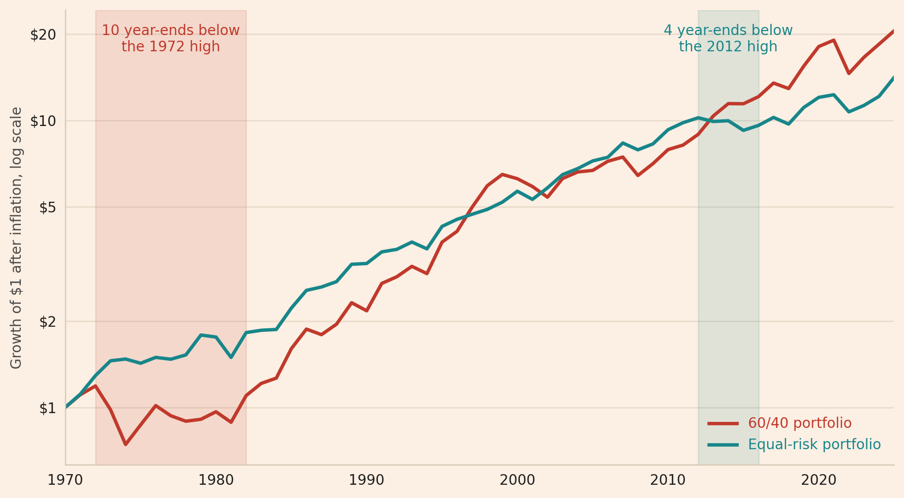
Read next
- Why the 60/40 portfolio is not dead How the measured risk of a 60/40 portfolio depends on how often its returns are measured.
- How did diversified portfolios do when US stocks rose or fell? Three diversified portfolios in the S&P 500’s rising and falling months since 1988.
- The Markowitz curse How raising one stock’s estimated volatility from 20% to 20.2% moves a minimum-variance weight from 50% to 99.5%.
Disclaimer: an explanation for teaching purposes, not investment advice. Past performance does not guarantee future returns.
Data: US stocks from Kenneth French’s data library, the 10-year Treasury yield (Federal Reserve Board) and US consumer prices (US Bureau of Labor Statistics) through FRED, and gold and the S&P GSCI Total Return index from LSEG Workspace (licensed). I do not reproduce the raw files here.
Sources: Bridgewater Associates, The All Weather Story, 2012. Marco Lombardi and Vladyslav Sushko, The correlation of equity and bond returns, BIS Quarterly Review, December 2023. Lasse Heje Pedersen, Efficiently Inefficient: How Smart Money Invests and Market Prices Are Determined, Princeton University Press, 2015, page 171. Claude B. Erb and Campbell R. Harvey, The Golden Dilemma, NBER Working Paper 18706, 2013. Sébastien Maillard, Thierry Roncalli and Jérôme Teïletche, The Properties of Equally Weighted Risk Contribution Portfolios, Journal of Portfolio Management 36(4), 60-70 (2010).