Buy the dip? US vs. Europe

I test buying a stock after its drawdown crosses a threshold and holding 12 months, across the US and 13 European markets. It roughly held in the US and got steadily worse across Europe.

Buying a US stock after a shallow fall from its own peak earned a small positive return over the next 12 months. Buying a European stock after the same shallow fall barely beat its own market, then fell steadily behind as the drawdown deepened. In the US the abnormal return is small and mostly positive at shallow drawdowns and fades toward zero as the drawdown deepens. In Europe it is negative from a 10% drawdown on and gets steadily worse.

I test whether buying the dip pays across markets. This extends an earlier post on buying US dips. That one bought after a fixed drop and looked only at the US. Here I use each stock’s drawdown from its own running peak, hold for 12 months, and run the same test on the US against a combined Europe of 13 countries.

The measure is the buy-and-hold abnormal return (BHAR). It is the stock’s compounded total return over the 12 months after the trigger, less the compounded return of its own market over those same days, less the round-trip trading cost. A positive BHAR means the dip-buyer beat the market net of costs.

The strategy

• Universe. US common stocks, 10,061 names, and 13 European markets, 9,971 names across GB, SE, FI, DK, NO, DE, FR, IT, NL, ES, BE, PT, and AT. Both include active and delisted stocks, through early 2026.
• Event. At each month-end, a stock’s drawdown from its own running peak crosses a threshold. I take one event per drawdown episode, the month it first crosses, and reset when the stock makes a new peak.
• Threshold. I run every threshold from 5% to 75% in 5-point steps.
• Hold. 252 trading days, about 12 months, buy and hold.
• Benchmark. Each stock against its own country’s value-weighted market. I pool European stocks only after measuring each against its home market.
• Costs. The bid-ask half-spread on entry and on exit, plus a 0.05% commission each way.

Starting point

The backtest runs off one price file per market. Building each file is a separate job that depends on the data vendor. I pull from LSEG Workspace. Because the data is licensed, the raw files stay off this page, and I show the code without running it here. I convert market caps to US dollars for comparison, GB through GBPUSD and the rest through EURUSD, using daily rates from the same source.

Step 1. Drawdown and events

Each stock carries a running peak. The drawdown is how far below that peak it currently sits.

HORIZON_DAYS = 252                              # hold for about 12 trading months
COMMISSION   = 0.0005                           # 0.05% each way

# Drawdown from each stock's own running peak.
df["ret_mult"] = 1 + df["ret"]
df["cum_ret"]  = df.groupby("Instrument")["ret_mult"].cumprod()
df["cum_max"]  = df.groupby("Instrument")["cum_ret"].cummax()
df["drawdown"] = df["cum_ret"] / df["cum_max"] - 1.0

I check the drawdown only at month-ends, so a stock triggers at most once a month. One drawdown episode gives one event, the first month it crosses the threshold. The episode closes when the stock reclaims a new peak, and only then can it trigger again.

def find_events(sd, thresh):
    """One event per drawdown episode: the month its drawdown first crosses -thresh."""
    dates, dds, month_ends = sd["dates"], sd["dds"], sd["month_ends"]
    events, in_episode = [], False
    for j in range(len(dates)):
        if dates[j] not in month_ends:          # only look at month-ends
            continue
        if dds[j] <= -thresh:
            if not in_episode:                  # first crossing of this episode
                in_episode = True
                if j + 1 < len(dates):
                    events.append(j + 1)        # buy at the next close, so the signal is lagged
        elif dds[j] >= 0:                       # back to a new peak: the episode resets
            in_episode = False
    return events

I read the event at the month-end close and buy at the following close, so the signal lags by one day and the test does not buy on information it could not have had. The reason to lag is in Lesson 30. I also drop any event whose 12-month window would run past the end of the sample, unless the stock delisted first, so the deep thresholds do not fill with holds cut short by the data ending.

Step 2. The abnormal return, net of costs

For each event I compound the stock over the next 252 days, compound its own market over the same days, and subtract. Then I take off the half-spread and commission to enter and to exit.

def bhar(sd, market, start_seq):
    """12-month buy-and-hold abnormal return for one event, net of costs."""
    rets, dates, spreads = sd["ret"], sd["dates"], sd["half_spread"]
    n_fwd = min(start_seq + HORIZON_DAYS, len(rets)) - start_seq

    stock = np.prod(1 + rets[start_seq:start_seq + n_fwd]) - 1     # the stock over 12 months
    mkt = 1.0
    for j in range(n_fwd):                                         # its own market, same days
        mkt *= 1 + market.get(dates[start_seq + j], 0.0)
    mkt -= 1

    entry, exit = spreads[start_seq], spreads[start_seq + n_fwd - 1]
    return stock - mkt - (entry + COMMISSION) - (exit + COMMISSION)

I value-weight the market return by the previous day’s market cap, so large stocks carry the benchmark. Where a European quote was missing or the bid and ask were swapped, I fill the half-spread with the median for that country and year, which keeps the cost estimate on the right scale for each market.

Step 3. Across every threshold and both markets

For each threshold I find the events, price each one, and take the median. US stocks go against the US market. European stocks go against their own country’s market first, and then I pool the abnormal returns into one European figure.

thresholds = np.arange(0.05, 0.80, 0.05)          # 5% to 75% in 5-point steps

for thresh in thresholds:
    # US: every stock against the US market.
    us_ev = [bhar(sd, us_mkt, s)
             for sd in us_sd.values() for s in find_events(sd, thresh)]

    # Europe: every stock against its OWN country's market, then pool the results.
    eu_ev = [bhar(sd, eu_data[code]["market_vw"], s)
             for code in eu_data
             for sd in eu_data[code]["stock_data"].values()
             for s in find_events(sd, thresh)]

    print(f"{int(thresh*100):>2d}%  "
          f"US {np.median(us_ev) * 100:+.1f}%  ({len(us_ev):,} events)  "
          f"EU {np.median(eu_ev) * 100:+.1f}%  ({len(eu_ev):,} events)")

 5%  US +6.8%  (33,737 events)  EU +1.3%  (27,337 events)
10%  US +6.8%  (26,651 events)  EU -2.1%  (22,183 events)
15%  US +5.7%  (21,544 events)  EU -6.6%  (18,627 events)
20%  US +3.8%  (17,922 events)  EU -11.2%  (16,149 events)
25%  US +2.5%  (15,413 events)  EU -14.6%  (14,420 events)
30%  US +0.5%  (13,453 events)  EU -16.4%  (13,086 events)
35%  US -0.1%  (11,951 events)  EU -18.6%  (11,980 events)
40%  US -0.6%  (10,665 events)  EU -19.7%  (11,044 events)
45%  US -1.5%  ( 9,611 events)  EU -20.3%  (10,229 events)
50%  US -2.4%  ( 8,708 events)  EU -20.4%  ( 9,453 events)
55%  US -2.6%  ( 7,803 events)  EU -21.2%  ( 8,718 events)
60%  US -2.4%  ( 6,992 events)  EU -21.8%  ( 8,003 events)
65%  US -1.7%  ( 6,230 events)  EU -21.8%  ( 7,341 events)
70%  US -2.4%  ( 5,533 events)  EU -21.2%  ( 6,652 events)
75%  US -1.4%  ( 4,849 events)  EU -23.1%  ( 6,031 events)

In the US the abnormal return is 6.8% after a 5% drawdown and 6.8% again after a 10% one. It falls as the drawdown deepens, reaches 0.5% at a 30% drawdown, and crosses zero around 35%. From there it stays mildly negative, at most 2.6% below the market at a 55% drawdown, and it is 1.4% below at a 75% drawdown.

Europe starts at 1.3% after a 5% drawdown and turns negative from 10% on. It then falls without recovering: 6.6% below the market at 15%, 11.2% below at 20%, 16.4% below at 30%, 20.4% below at 50%, and 23.1% below at a 75% drawdown. So, in Europe a deeper dip tends to mean a worse 12 months, and the shortfall deepens across almost the whole range.

Results

Median 12-month abnormal return after a drawdown, US against Europe, by drawdown threshold. The US line stays near zero across the range, while the Europe line falls steadily as the drawdown deepens.

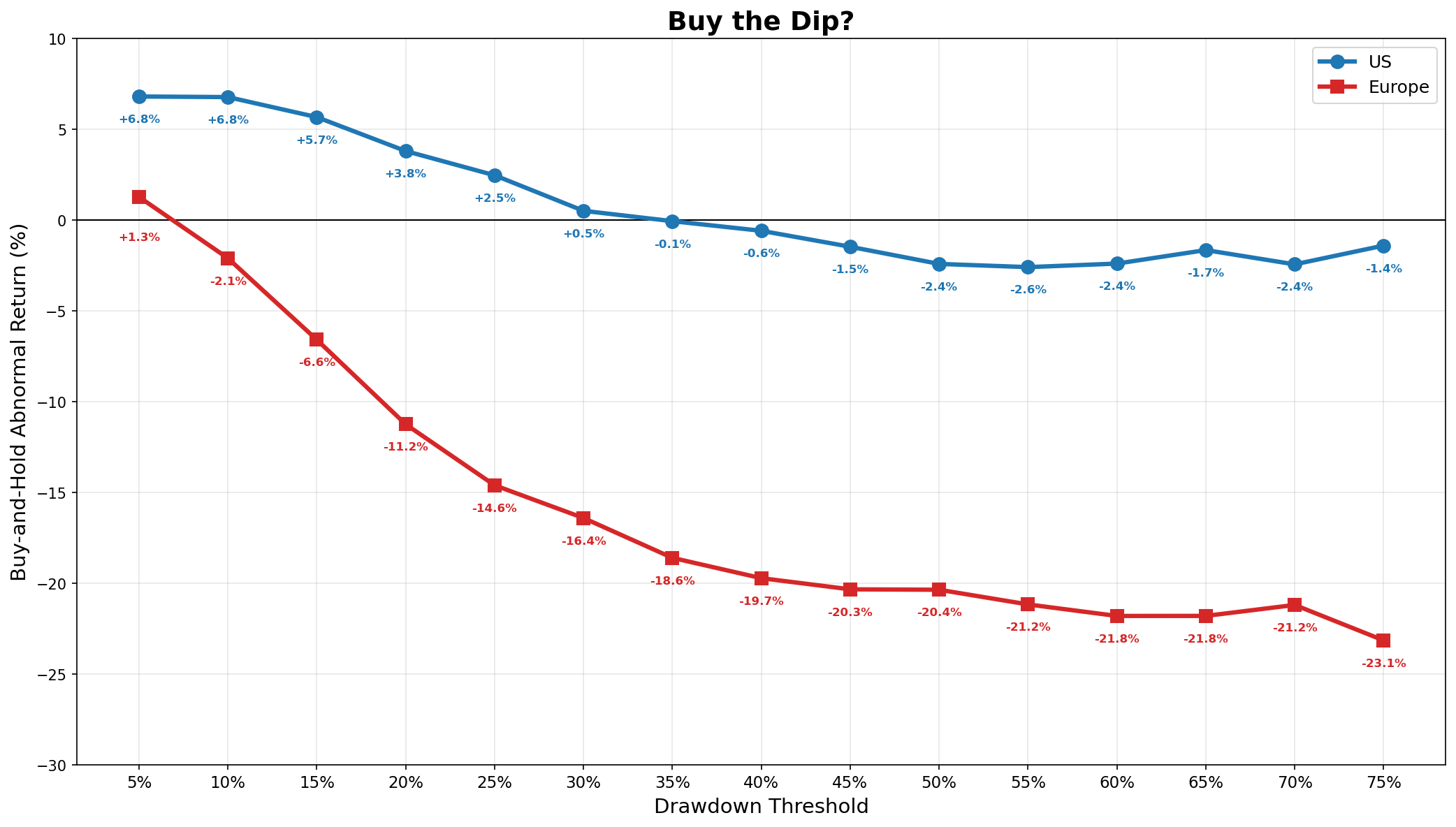
The two lines separate immediately and never cross back. The US line hovers near the market at every threshold, a few points above it for shallow dips and a few points below it for deep ones. The European line heads down and keeps going.

The European stocks that trigger are smaller and cost more to trade, which is part of the gap. At a 5% drawdown the median US trigger was a 742 million dollar company with a 0.1% half-spread. The median European trigger was a 271 million dollar company with a 0.7% half-spread. At a 75% drawdown the US median fell to 185 million and the European to 32 million, and the European half-spread rose to 1.3% while the US one reached 0.3%. So, a European dip-buyer holds smaller, thinner names and pays more each time to get in and out.

What this test does not settle

Each stock against its own market. The BHAR is relative to the home benchmark, so a negative European figure says the dip stock trailed its own rising or falling market. It does not measure the absolute return of buying the dip, and a market that itself fell hard would flatter the comparison.

Costs are approximate. The half-spread plus a flat commission understates real trading costs, and slippage is worse in small, thin names, which the deep thresholds hold. I fill many European spreads with a country-year median where quotes were missing or swapped, so the European cost is an estimate and the true drag on deep European dips is probably higher than charged here.

The events are not independent. Drawdowns cluster in bear markets, so a single bad year like 2008 or 2020 fills many events at once. The 392-thousand-odd events are not that many separate experiments, and I do not attach a confidence interval to any single figure.

It is a per-event median. Each number is the middle event at that threshold. Turning it into a portfolio return would need position sizing and would have to handle the overlap between events, which this test does not model.

What it means

Buying the dip behaved differently on the two continents. In the US the rule stayed close to the market across the whole range, a little ahead after shallow falls and a little behind after deep ones. In Europe it trailed the market from a 10% drawdown on and trailed further at every deeper level, down to 23.1% below after a 75% fall. The European dip stocks are smaller and dearer to trade, and their returns after a deep drawdown did not recover the ground. The takeaway is that buying the dip did not travel, because a rule that was roughly flat in the US turned steadily costly across Europe as the drawdown deepened.

Read next

• Does a Large One-Day Move in the S&P 500 Predict Next Week’s Return? The earlier US dip test that prompted this comparison.
• Should you wait for new lows or new highs? The other side of the timing instinct: what waiting for a signal costs a steady saver.

Disclaimer: simplified, hypothetical backtest with approximate trading costs, for discussion purposes only. Not investment advice. Past performance does not predict future returns.

Data: US and European equity total returns, bid-ask quotes, and market caps from LSEG Workspace (licensed), with EURUSD and GBPUSD from the same source for currency conversion. I benchmark each stock against its own country’s value-weighted market. I do not reproduce the raw file here.