Six ways to clean your trading data into the wrong answer

Six ordinary processing steps, each measured against a truth known by construction. One dropna call takes a third off the terminal wealth, and a missing delisting return adds 73.1%.

We download a price panel, find gaps in it, and clean them out with dropna(). The issue, however, is that as the gaps go, so do returns that, in truth, were not missing. Dropping a row removes every asset on that row, including the ones that reported.

In this post I run six ordinary processing steps on data I simulate myself, so the true result is known in advance. Each runs without an error and returns plausible statistics. One dropna() call takes a third off the terminal wealth. A missing delisting return adds 73.1%.

That comes at a cost. The sizes below hold for these simulations. On real equity, bond, gold, and crypto data the same mistakes would give different numbers, because what they cost depends on which assets are held and over what period.

Sections 1 to 3 are three mistakes hiding inside a single dropna() call on one simulated market. Sections 4, 5 and 6 each have a simulation of their own.

1. Dropping a row deletes every asset on it

Three assets in a DataFrame, and one of them has no value on the Tuesday.

import numpy as np, pandas as pd

demo = pd.DataFrame({"Equity": [0.010,  0.020, -0.010],
                     "Gold":   [0.005, np.nan,  0.007],   # Gold did not report on Tuesday
                     "Bonds":  [0.002,  0.001,  0.003]},
                    index=["Monday", "Tuesday", "Wednesday"])
print("what we downloaded"); print(demo.to_string())
print("\nafter .dropna()");  print(demo.dropna().to_string())

what we downloaded
           Equity   Gold  Bonds
Monday       0.01  0.005  0.002
Tuesday      0.02    NaN  0.001
Wednesday   -0.01  0.007  0.003

after .dropna()
           Equity   Gold  Bonds
Monday       0.01  0.005  0.002
Wednesday   -0.01  0.007  0.003

Tuesday is gone, and Equity’s +2.0% and Bonds’ +0.1% went with it. Neither was missing. DataFrame.dropna() removes the whole row when any column holds an NA, which is what it documents.

2. Cleaning a price series merges two days into one

I apply the same cleaning to the prices instead of the returns.

px = pd.Series([100.0, np.nan, 105.0], index=["Monday", "Tuesday", "Wednesday"])
print(px.dropna().pct_change().to_string())      # the usual clean-then-difference idiom

Monday        NaN
Wednesday    0.05

Wednesday reads +5.0%, and the price move did end on Wednesday. It is a two-day return in a series of one-day returns. pct_change() compares each row with the previous surviving row rather than the previous calendar day. Every rolling window downstream now treats an unequal gap as an equal one. Lesson 17 covers pct_change() on a price series.

Whether that matters depends on what the NA meant, and three cases look identical in a DataFrame.

The market was closed. Nothing traded anywhere, so no return existed for anyone. Compounding across the closure is correct.

The asset trades on a different calendar. Bitcoin trades at the weekend and equities do not. The return is real for bitcoin on that row, and there was never one to record for the rest.

The vendor failed to send it. Every asset traded, and the vendor lost one of the returns. Deleting that row throws away the ones it did send.

3. A weekend is not a missing day

Real data does not label which case an NA belongs to, though much of it can be worked out. A business-day calendar separates a closure from a gap. An asset that reported when the others did not points at the vendor. The return the vendor dropped is gone either way, so there is nothing to measure the error against. A simulation keeps it, since we built it.

In the following, I build four (fake) assets over twenty years. Equity, Bonds, and Gold trade Monday to Friday, and Crypto trades every day. I also assume that the vendor we get the data from drops a scheduled observation now and then, most often for Gold.

SEED, START, END = 12, "2006-01-01", "2026-01-01"
ASSETS = {  # annual drift, annual volatility, native calendar, P(vendor drops a day)
    "Equity": dict(mu=.08, sd=.16, cal="B", miss=.000),
    "Bonds":  dict(mu=.03, sd=.05, cal="B", miss=.015),
    "Gold":   dict(mu=.04, sd=.15, cal="B", miss=.040),
    "Crypto": dict(mu=.20, sd=.45, cal="D", miss=.005)}
W   = pd.Series({"Equity": .45, "Bonds": .30, "Gold": .15, "Crypto": .10})
RHO = np.array([[1, -.2, .1, .35], [-.2, 1, .15, 0], [.1, .15, 1, .1], [.35, 0, .1, 1]])

cal = pd.date_range(START, END, freq="D")        # every calendar day
biz = pd.date_range(START, END, freq="B")        # Monday to Friday
names, YRS = list(ASSETS), (cal[-1] - cal[0]).days / 365.25

rng = np.random.default_rng(SEED)                # fixed, so the post reproduces
Z = pd.DataFrame(rng.standard_normal((len(cal), 4)) @ np.linalg.cholesky(RHO).T,
                 index=cal, columns=names)
latent, true_px = {}, {}
for a in names:
    p, d = ASSETS[a], (biz if ASSETS[a]["cal"] == "B" else cal)
    py = len(d) / YRS                            # what this calendar delivers in a year
    latent[a]  = p["mu"]/py - .5*p["sd"]**2/py + p["sd"]/np.sqrt(py)*Z.loc[d, a]
    true_px[a] = 100*np.exp(latent[a].cumsum())

r, obs = np.random.default_rng(SEED + 1), {}     # what we actually download
for a in names:
    s = true_px[a]; k = r.random(len(s)) >= ASSETS[a]["miss"]; k[0] = k[-1] = True
    for e in (biz[0], biz[-1]):
        if e in s.index: k[s.index.get_loc(e)] = True
    obs[a] = s[k]
    print(f"  {a:7s} traded {len(s):5,}   reported {len(obs[a]):5,}   "
          f"vendor gaps {len(s)-len(obs[a]):4,} ({1-len(obs[a])/len(s):.2%})")

import sys, matplotlib
print(f"\n  python {sys.version.split()[0]} | numpy {np.__version__} | "
      f"pandas {pd.__version__} | matplotlib {matplotlib.__version__}")

  Equity  traded 5,219   reported 5,219   vendor gaps    0 (0.00%)
  Bonds   traded 5,219   reported 5,139   vendor gaps   80 (1.53%)
  Gold    traded 5,219   reported 5,020   vendor gaps  199 (3.81%)
  Crypto  traded 7,306   reported 7,269   vendor gaps   37 (0.51%)

  python 3.13.1 | numpy 2.4.2 | pandas 2.3.3 | matplotlib 3.10.8

Under 4% of Gold’s days are missing and the other three are cleaner. I fix the seed and print the package versions, so these are the numbers you get too.

Here is what dropna() does to six weeks of it.

import matplotlib.pyplot as plt
from matplotlib.patches import Patch, Rectangle

BLUE, RED, AMBER, CLOSED = "#4C72B0", "#C44E52", "#E1A100", "#b5b5b5"
INK, MUTED, GRID = "#2b2b2b", "#767676", "#e8e8e8"
DAY = pd.Timedelta("1D")
win = pd.date_range("2006-02-06", periods=42, freq="D")          # six weeks
state = pd.DataFrame({a: ["reported" if d in set(obs[a].index) else
                          "lost" if d in set(true_px[a].index) else "closed" for d in win]
                      for a in names}, index=win).T
keep = pd.Series({d: (state[d] == "reported").all() for d in win})
COLOUR = {"reported": BLUE, "closed": CLOSED, "lost": RED}

fig, ax = plt.subplots(figsize=(12.5, 4.3))
for d in win[~keep.values]:                      # a dark bar marks every day .dropna() removes
    ax.add_patch(Rectangle((d-.40*DAY, -.92), .8*DAY, .30, facecolor=INK,
                           edgecolor="white", lw=1, zorder=3))
ax.text(win[0]-.75*DAY, -.77, "deleted", ha="right", va="center", fontsize=10.5,
        color=INK, fontweight="bold")
for i, a in enumerate(names):
    for d in win:
        ax.add_patch(Rectangle((d-.40*DAY, 3-i-.33), .8*DAY, .66,
                               facecolor=COLOUR[state.loc[a, d]],
                               edgecolor="white", lw=1, zorder=3))
ax.annotate("Bonds is missing here, so Equity, Gold\nand Crypto lose this day as well",
            xy=(pd.Timestamp("2006-02-13"), 3.40),
            xytext=(pd.Timestamp("2006-02-13")+2.2*DAY, 4.15), fontsize=10.5, color=INK,
            ha="left", va="bottom",
            arrowprops=dict(arrowstyle="-", color=MUTED, lw=1.1,
                            connectionstyle="angle,angleA=0,angleB=90,rad=4"))
ax.set_xlim(win[0]-.7*DAY, win[-1]+.7*DAY); ax.set_ylim(-1.15, 4.7)
ax.set_yticks(range(4)); ax.set_yticklabels(names[::-1], fontsize=11)
mon = [d for d in win if d.dayofweek == 0]
ax.set_xticks(mon); ax.set_xticklabels([d.strftime("%d %b") for d in mon], fontsize=10)
ax.tick_params(length=0, colors=INK)
for sp in ax.spines.values(): sp.set_visible(False)
ax.set_title("What .dropna() deletes",
             fontsize=13.5, fontweight="bold", pad=16, loc="left")
ax.legend(handles=[Patch(facecolor=BLUE, label="reported"),
                   Patch(facecolor=CLOSED, label="market closed"),
                   Patch(facecolor=RED, label="vendor lost it"),
                   Patch(facecolor=INK, label="day deleted by .dropna()")],
          frameon=False, fontsize=10.5, ncol=4, loc="lower left", bbox_to_anchor=(-.005, -.30))
plt.tight_layout()
fig.savefig("dc_what_dropna_deletes.png", dpi=200, bbox_inches="tight", facecolor="white")
plt.show()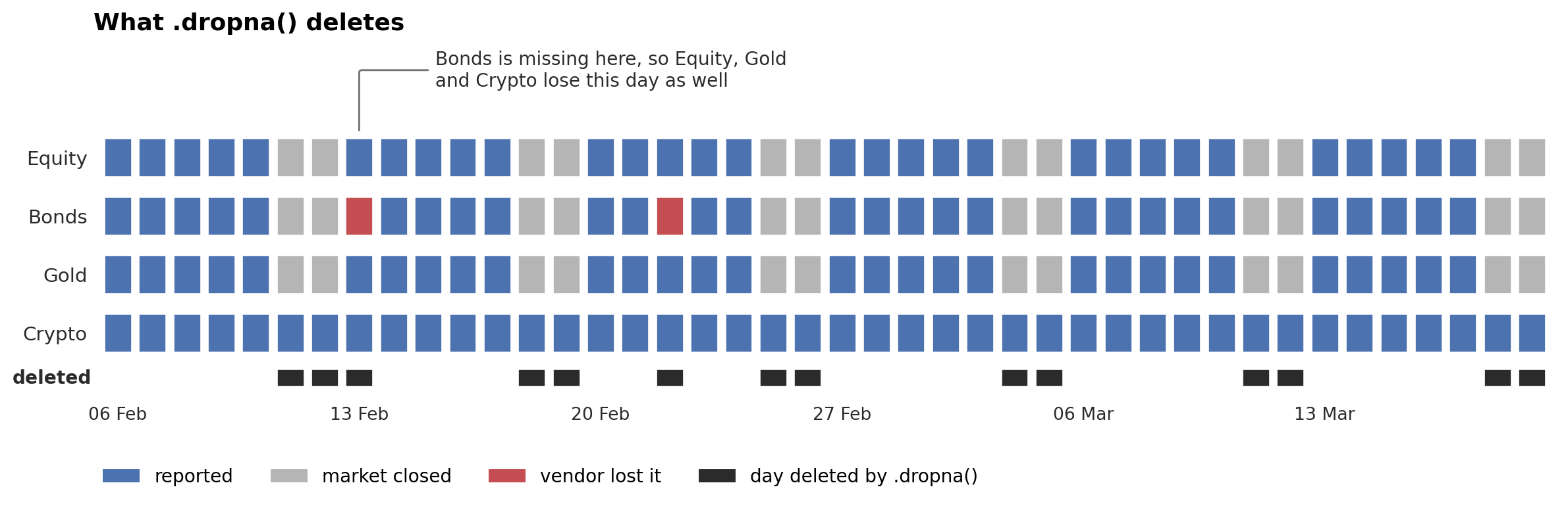

Each cell is one asset on one day. Grey means the market was shut, red means the vendor lost the day, and a dark bar underneath marks a day dropna() deletes.

Most of the deleted days are weekends. Crypto traded and the others did not, so those returns are deleted instead of compounded into the Friday-to-Monday move. The rest are days holding one red cell, where a single asset failed to report and the whole day went with it.

Then I repair the pipeline one mistake at a time, on the prices rather than the returns. I build each wealth index on the asset’s own dates, carry it forward to the valuation days, and difference it there.

def on_cal(px, dates):
    # carry the last known price across days the asset did not trade or did not report
    return px.reindex(px.index.union(dates)).ffill().reindex(dates)

true_r = pd.DataFrame({a: on_cal(true_px[a], biz).pct_change() for a in names}).dropna()
step1  = pd.DataFrame({a: obs[a].dropna().pct_change() for a in names}).dropna()
step2  = pd.DataFrame({a: (on_cal(obs[a], biz).pct_change() if ASSETS[a]["cal"] == "B"
                           else on_cal(obs[a], cal).pct_change().reindex(biz))
                       for a in names}).dropna()
step3  = pd.DataFrame({a: on_cal(obs[a], biz).pct_change() for a in names}).dropna()

SPAN1 = (true_r.index[-1] - biz[0]).days / 365.25   # the calendar span every version covers
PPY1  = len(true_r) / SPAN1                         # 261 business days a year here, not 252

def stats(r):
    # every version is scored on the same valuation calendar, with a zero on any day it
    # deleted. That stops a series with fewer rows being annualised on a slower clock.
    r   = r.reindex(true_r.index).fillna(0.0)
    tot = float((1 + r).prod())
    w   = np.r_[1.0, (1 + r).cumprod().values]
    return (tot, tot**(1/SPAN1) - 1, r.std(ddof=1)*np.sqrt(PPY1),
            r.mean()/r.std(ddof=1)*np.sqrt(PPY1), float((w/np.maximum.accumulate(w) - 1).min()))

LADDER = [("1  .dropna() on everything",   step1), ("2  + stop deleting whole rows", step2),
          ("3  + compound the weekend in", step3), ("   the truth",                 true_r)]
T = stats(true_r @ W)[0]
print(f"{'':32s}{'wealth':>9}{'error':>9}{'CAGR':>8}{'vol':>8}{'Sharpe':>9}{'max DD':>9}")
for lab, pnl in LADDER:
    tot, cagr, vol, shp, dd = stats(pnl @ W)
    err = "" if "truth" in lab else f"{tot/T-1:+.1%}"
    print(f"{lab:32s}{tot:>8.2f}x{err:>9}{cagr:>8.2%}{vol:>8.2%}{shp:>9.2f}{dd:>9.1%}")

crr  = true_px["Crypto"].pct_change().dropna()
crr  = crr[crr.index > biz[0]]
wknd = int((~crr.index.isin(biz)).sum())
kept = int(crr.index.isin(step1.index).sum())
print(f"\nCrypto has {len(crr):,} returns inside the portfolio's horizon and {kept:,} survive")
print(f"  {wknd:,} ({wknd/len(crr):.1%}) fall at a weekend")
print(f"  {len(crr)-kept-wknd:,} ({(len(crr)-kept-wknd)/len(crr):.1%}) fall on a business day "
      f"where some asset had a vendor gap")

                                   wealth    error    CAGR     vol   Sharpe   max DD
1  .dropna() on everything          3.82x   -32.9%   6.94%   9.61%     0.75   -19.4%
2  + stop deleting whole rows       4.63x   -18.9%   7.96%   9.88%     0.82   -16.3%
3  + compound the weekend in        5.70x    +0.0%   9.10%  10.24%     0.90   -16.4%
   the truth                        5.70x            9.10%  10.25%     0.90   -16.4%

Crypto has 7,304 returns inside the portfolio's horizon and 4,916 survive
  2,086 (28.6%) fall at a weekend
  302 (4.1%) fall on a business day where some asset had a vendor gap

dropna() on everything reports 3.82x against a true 5.70x, an error of 32.9%. Step 2 closes about two fifths of that, and step 3 lands within 0.05% of the truth.

STEPS = [(step1, RED, "-", "1  .dropna() on everything"), (step2, AMBER, "-", "2  + stop deleting whole rows"),
         (step3, BLUE, "--", "3  + compound the weekend in"), (true_r, INK, "-", "   the truth")]
PAD = max(len(l) for *_, l in STEPS) + 4
fig, ax = plt.subplots(figsize=(11.5, 5.6))
for pnl, colour, ls, lab in STEPS:
    w = (1 + pnl @ W).cumprod()
    ax.plot(w.index, w.values, color=colour, ls=ls, lw=2.1, solid_capstyle="round",
            zorder=5 if ls == "--" else 3, label=f"{lab:<{PAD}}{w.iloc[-1]:.2f}x")
ax.set_xlim(true_r.index[0], true_r.index[-1])
ax.set_ylabel("Value of 1.00 invested", fontsize=11, color=INK)
ax.set_title("One history, processed four ways", fontsize=13.5,
             fontweight="bold", pad=16, loc="left")
ax.legend(frameon=False, loc="upper left", labelcolor=INK,
          prop={"family": "monospace", "size": 10.5}, handlelength=2.4, labelspacing=.55)
ax.grid(True, color=GRID, lw=.8); ax.set_axisbelow(True)
ax.tick_params(labelsize=10, colors=MUTED, length=0)
for sp in ("top", "right"): ax.spines[sp].set_visible(False)
for sp in ("left", "bottom"): ax.spines[sp].set_color(GRID)
plt.tight_layout()
fig.savefig("dc_wealth_paths.png", dpi=200, bbox_inches="tight", facecolor="white")
plt.show()

same = int((np.abs(step3.values - true_r.values) < 1e-12).all(axis=1).sum())
gapw = ((1 + step3 @ W).cumprod() / (1 + true_r @ W).cumprod() - 1)
print(f"daily returns identical to the truth: {same:,} of {len(step3):,}")
print(f"the wealth path runs between {gapw.min():+.2%} and {gapw.max():+.2%} "
      f"before ending {gapw.iloc[-1]:+.3%} away")

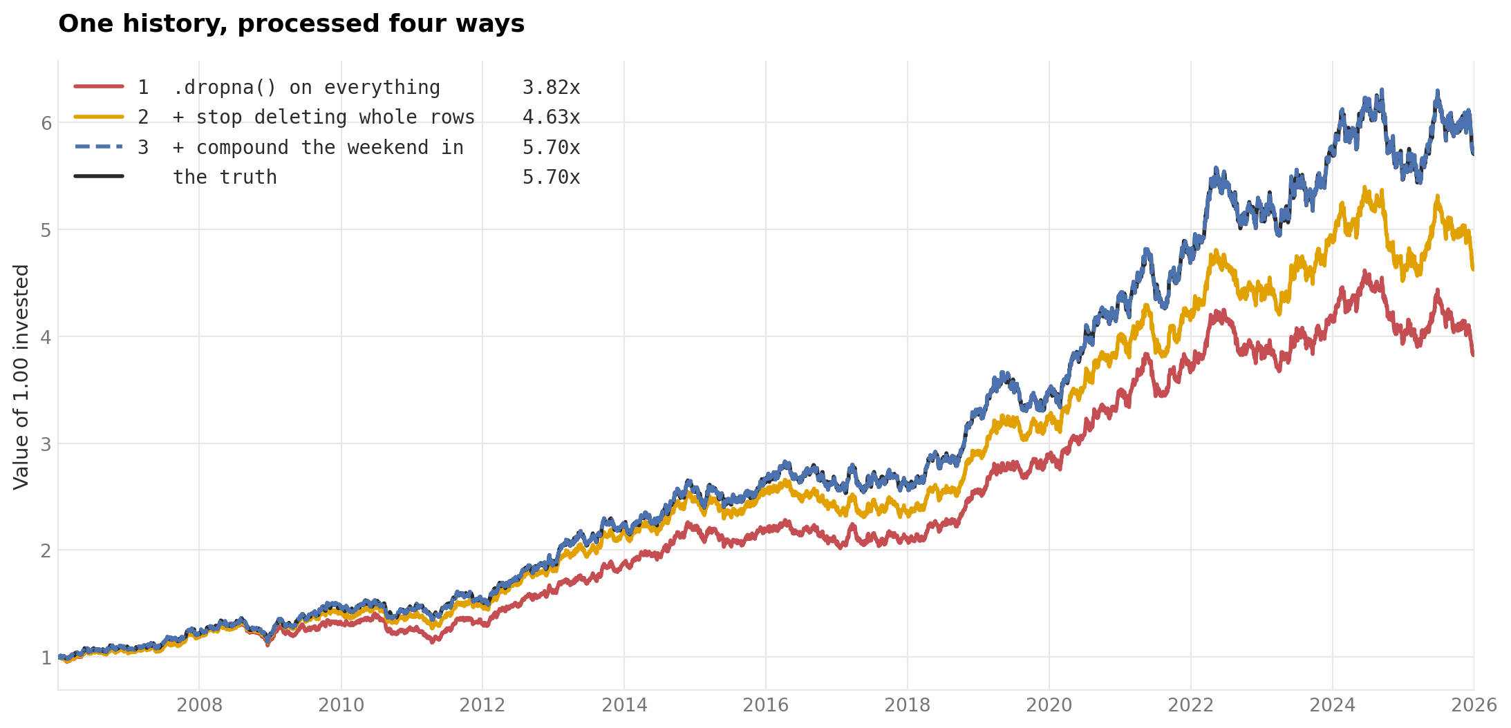
daily returns identical to the truth: 4,630 of 5,218
the wealth path runs between -0.83% and +0.49% before ending +0.048% away

The black line is the truth, and the blue dashed version sits on top of it.

So, neither repair is enough alone. Step 2 is still 19% below the truth. Its row count matches all 5,218 business-day intervals exactly, so counting rows would not catch it. Step 3 recovers the level. It does not recover the timing, and only 4,630 of the 5,218 daily returns match exactly.

Those are three mistakes inside one call, so I measure each alone with the other two handled correctly.

gapdays = pd.Index(sorted(set().union(*[set(true_px[a].index) - set(obs[a].index)
                                        for a in names]))).intersection(true_r.index)
A = true_r.drop(index=gapdays)                     # rows deleted from a table of returns
B = step3                                          # prices repaired, the gap still mis-timed
C = pd.DataFrame({a: (on_cal(true_px[a], biz).pct_change() if ASSETS[a]["cal"] == "B"
                      else true_px[a].pct_change().reindex(biz))
                  for a in names}).dropna()        # no gaps at all, weekend thrown away

CASE = {}   # label -> (list of (naive, matching truth) pairs, periods a year, years spanned)
zf = lambda x: x.reindex(true_r.index).fillna(0.0)          # one clock for both sides
CASE["1  rows deleted by .dropna()"]      = ([(zf(A @ W), true_r @ W)], PPY1, SPAN1)
CASE["2  a gap merged into the next day"] = ([(B @ W,     true_r @ W)], PPY1, SPAN1)
CASE["3  weekend returns discarded"]      = ([(C @ W,     true_r @ W)], PPY1, SPAN1)
print(f"{len(gapdays)} of {len(true_r):,} valuation days carried a vendor gap somewhere\n")
for k, (pairs, *_) in CASE.items():
    n, t = pairs[0]
    print(f"  {k:36s}{float((1+n).prod())/float((1+t).prod())-1:>+9.2%}")

302 of 5,218 valuation days carried a vendor gap somewhere

  1  rows deleted by .dropna()          -23.25%
  2  a gap merged into the next day      +0.05%
  3  weekend returns discarded          -17.77%

Deleting rows costs 23.25%. Discarding the weekend costs 17.77%. The mis-timed gap costs 0.05%, because this history happens to end where the mis-timings cancel. The three do not add up to 32.9%. Each answers what one mistake costs alone.

4. Panel operations do not know what a stock is

A long panel is one row per stock per day, and these are the obvious two lines.

df["ret"] = df["Price"].pct_change()
df["sig"] = df["ret"].rolling(21).sum()

The issue is that both compare each row with the rows above it, which in a long panel are often a different company. I simulate forty stocks that, in truth, have no edge at all. They list on different dates the way a real universe fills up, and I run a 21-day momentum strategy on top.

g2 = np.random.default_rng(4); NS, ND, N2 = 40, 2520, 8
tick = [f"STK{i:02d}" for i in range(NS)]; idx2 = pd.bdate_range("2014-01-01", periods=ND)
lvl = g2.uniform(5, 500, NS); rr = g2.normal(0, .02, (ND, NS))
listing = np.sort(g2.integers(0, 1200, NS)); listing[:12] = 0   # the universe fills up over time
px2 = pd.DataFrame(lvl*np.exp(np.cumsum(rr - .5*.02**2, axis=0)), index=idx2, columns=tick)
for j, s0 in enumerate(listing): px2.iloc[:s0, j] = np.nan
PPY2 = (ND - 1) / ((idx2[-1] - idx2[0]).days / 365.25)
# .dropna() removes the pre-listing cells on every pandas version, including 3.x,
# where stack() stops removing them for us
long = (px2.stack().dropna().rename("Price").reset_index()
           .rename(columns={"level_0": "Date", "level_1": "Ticker"}))

def build(df, gret, groll):        # the two lines can be got wrong independently
    d = df.sort_values(["Ticker", "Date"]).reset_index(drop=True)
    d["ret"] = (d.groupby("Ticker", observed=True)["Price"].pct_change() if gret
                else d["Price"].pct_change())
    d["sig"] = (d.groupby("Ticker", observed=True)["ret"].rolling(21).sum()
                 .reset_index(level=0, drop=True) if groll else d["ret"].rolling(21).sum())
    return d

def mom(d, n=N2):                  # long the top n, short the bottom n, on yesterday's signal
    w  = d.pivot_table(index="Date", columns="Ticker", values="ret")
    rk = d.pivot_table(index="Date", columns="Ticker", values="sig").shift(1).rank(axis=1)
    rk = rk.reindex(columns=w.columns); cnt = rk.notna().sum(axis=1)
    pos = (rk.gt(cnt-n, axis=0).astype(float) - (rk <= n).astype(float)).div(2*n)
    pos = pos.where(cnt >= 2*n, 0.0)
    return (pos*w).sum(axis=1, min_count=1).where(pos.abs().sum(axis=1) > 0).dropna()

FOUR = {(gr, gl): mom(build(long, gr, gl)) for gr in (True, False) for gl in (True, False)}
ok   = FOUR[(True, True)]; common = ok.index
flat = build(long, False, False)
cross = int((flat["Ticker"].shift(1).notna()
             & (flat["Ticker"].shift(1) != flat["Ticker"]) & flat["ret"].notna()).sum())
print(f"returns that compare two different companies: {cross} of {len(long)-1:,}\n")
for lab, key in [("both grouped (correct)", (True, True)), ("pct_change ungrouped", (False, True)),
                 ("rolling ungrouped",      (True, False)), ("both ungrouped",       (False, False))]:
    pl = FOUR[key].reindex(common)
    n  = int((~np.isclose(pl.values, ok.values, equal_nan=True)).sum())
    print(f"  {lab:24s}terminal {float((1+pl).prod()):.4f}x"
          f"{float((1+pl).prod())/float((1+ok).prod())-1:>9.1%}   trading days changed {n:>4}")

bad = FOUR[(False, False)].reindex(common)
CASE["4  ungrouped panel operations"] = ([(bad, ok)], PPY2, len(common)/PPY2)

# tickers are only labels, so relabelling them cannot change a correct result
perm = dict(zip(tick, list(np.random.default_rng(7).permutation(tick))))
sh = long.assign(Ticker=long["Ticker"].map(perm))
for lab, grp in [("grouped (correct)", True), ("ungrouped", False)]:
    a_, b_ = FOUR[(grp, grp)].reindex(common), mom(build(sh, grp, grp)).reindex(common)
    n = int((~np.isclose(a_.values, b_.values, equal_nan=True)).sum())
    print(f"  relabel test  {lab:20s}{'PASS' if n == 0 else 'FAIL'}   "
          f"days that move {n:>5,} of {len(common):,}")

returns that compare two different companies: 39 of 79,794

  both grouped (correct)  terminal 0.9327x     0.0%   trading days changed    0
  pct_change ungrouped    terminal 0.9415x     0.9%   trading days changed   24
  rolling ungrouped       terminal 0.9327x     0.0%   trading days changed    0
  both ungrouped          terminal 0.8796x    -5.7%   trading days changed  396
  relabel test  grouped (correct)   PASS   days that move     0 of 2,084
  relabel test  ungrouped           FAIL   days that move   213 of 2,084

Thirty-nine of the eighty thousand returns compare two different companies. The stocks list on different dates, so those thirty-nine fall mid-sample while the rest of the book is trading.

The four rows below matter more than that count. Ungrouped rolling() alone changes nothing. groupby().pct_change() leaves an NA on each stock’s first day, and any window crossing a company boundary returns NA too. Ungrouped pct_change() alone even helps. Only both together move the result, and terminal wealth falls 5.7%. So, this is a compound error, and fixing either line alone would have said the code was fine.

The relabelling test is the cheapest check here. Tickers are labels, so renaming them cannot change a correct result. The grouped version does not move, and the ungrouped one moves on 213 of 2,084 days. Lesson 22 covers groupby() and Lesson 25 the long panel.

5. The return after the last price

A database can hold every company that ever listed and still miss the last return, because it stops at the last price it observed. Shumway (1997) puts that missing return near -30% on NYSE and AMEX, and Shumway and Warther (1999) near -55% on Nasdaq, on 5.6% of stocks a year against 1.2%.

I simulate 300 firms over twenty years. I assume the chance of delisting rises after a poor twelve months, and that every exit is a performance-related delisting.

NF3, NM3, FAC, IDIO = 300, 240, .042, .080

def universe(seed, base, slope):
    r = np.random.default_rng(seed)
    # a common factor plus firm-specific noise. Without the factor, 300 equal-weighted
    # firms diversify away almost all risk and the portfolio Sharpe ratio means nothing.
    mret = r.normal(.006, FAC, (NM3, 1)) + r.normal(0, IDIO, (NM3, NF3))
    cs = np.vstack([np.zeros(NF3), np.cumsum(mret, axis=0)]); t = np.arange(NM3)
    H = base + slope*np.maximum(0., -(cs[t] - cs[np.maximum(t-12, 0)]))   # a bad year hurts
    H[:12] = 0.
    hit = r.random((NM3, NF3)) < H
    dl = np.where(hit.any(axis=0), hit.argmax(axis=0), -1)
    live = np.ones((NM3, NF3), bool)
    for j in range(NF3):
        if dl[j] >= 0: live[dl[j]+1:, j] = False
    return mret, dl, live

def three(mret, dl, live, dlret):
    truth = mret.copy()
    for j in range(mret.shape[1]):
        if dl[j] >= 0:                              # the delisting return compounds WITH the
            t = dl[j]                               # month's return, it does not replace it
            truth[t, j] = (1 + mret[t, j])*(1 + dlret) - 1
    surv = np.zeros_like(live); surv[:, dl < 0] = live[:, dl < 0]
    ew = lambda R, m: np.array([R[t][m[t]].mean() if m[t].any() else 0. for t in range(NM3)])
    return ew(truth, live), ew(mret, live), ew(mret, surv)

for tag, base, slope, dlret in [("Nasdaq   ", .00145, .036, -.55),
                                ("NYSE/AMEX", .00031, .0077, -.30)]:
    m3, d3, l3 = universe(11, base, slope)
    a_, b_, c_ = three(m3, d3, l3, dlret)
    wa, wb, wc = (float((1+x).prod()) for x in (a_, b_, c_))
    at_risk = sum((d3[j] if d3[j] >= 0 else NM3-1) - 11 for j in range(NF3))
    print(f"{tag}  {int((d3>=0).sum())} of {NF3} firms delisted "
          f"({(d3>=0).sum()/(at_risk/12):.2%} a year), delisting return {dlret:.0%}")
    print(f"    truth {wa:5.2f}x  |  delisting return missing {wb:5.2f}x ({wb/wa-1:+6.1%})"
          f"  |  survivors only {wc:5.2f}x ({wc/wa-1:+6.1%})")
    if tag.startswith("Nasdaq"):                    # only one calibration goes on the chart
        CASE["5  delisting return missing"] = ([(pd.Series(b_), pd.Series(a_))], 12, NM3/12)

Nasdaq     190 of 300 firms delisted (5.07% a year), delisting return -55%
    truth  1.98x  |  delisting return missing  3.43x (+73.1%)  |  survivors only  4.51x (+127.7%)
NYSE/AMEX  49 of 300 firms delisted (0.93% a year), delisting return -30%
    truth  3.34x  |  delisting return missing  3.52x ( +5.6%)  |  survivors only  3.71x (+11.1%)

The middle number, +73.1%, is the one to look at. It is not survivorship bias. That portfolio holds every firm including the ones that delisted, and it drops nothing. No missing row anywhere warns us. The survivors-only column beside it is plain survivorship bias. That error is larger and better known, which is why it is not one of the six.

The size of that error depends on the market: 73.1% at Nasdaq frequency and severity, 5.6% on NYSE and AMEX. One limit, because I apply the correction to every exit. Acquisitions are not in this simulation and must never receive it, because a firm bought by someone else carries no large negative return.

6. The date on the statement is not when the market knew

I end every fiscal year on 31 December. I assume the accounts appear two to four months later, and that for about a third of firms the reported number is revised again four to nine months after that. Many databases write the new value over the old. That is two leaks: using the figure before publication, and using a version nobody could have seen.

NF4, NY4, BETA4, NPOS = 400, 20, .0015, 60
T4 = NY4*12; cols = np.arange(NF4); mrow = np.arange(T4)[:, None]
fyr = mrow//12; into = mrow - fyr*12

def economy(seed):
    r = np.random.default_rng(seed)
    q   = r.normal(0, 1, (NY4, NF4))                # the firm-year's true quality
    lag = r.integers(2, 5, (NY4, NF4))              # months from year end to first release
    gap = r.integers(4, 10, (NY4, NF4))             # months from release to the revision
    upd = r.random((NY4, NF4)) < .35                # only a minority are ever revised
    rep = q + r.normal(0, .9, (NY4, NF4))           # the figure as FIRST reported
    fin = np.where(upd, q + r.normal(0, .3, (NY4, NF4)), rep)   # the value on file today
    mr  = r.normal(.005, .055, (T4, NF4))
    for y in range(NY4): mr[y*12:(y+1)*12] += BETA4*q[y]
    return lag, gap, rep, fin, mr

def vintage(rep, fin, lag, gap, mode):
    yv = np.where(into >= lag[fyr, cols], fyr, fyr-1) if mode != "fyend" else fyr
    ok_, yc = yv >= 0, np.clip(yv, 0, None)
    if mode != "pit":
        return np.where(ok_, fin[yc, cols], np.nan)
    at = 12*yc + lag[yc, cols] + gap[yc, cols]      # availability in absolute time
    return np.where(ok_, np.where(mrow >= at, fin[yc, cols], rep[yc, cols]), np.nan)

def rungs(seed):
    lag, gap, rep, fin, mr = economy(seed)
    raw = {}
    for m_ in ("fyend", "release", "pit"):
        Sd = pd.DataFrame(vintage(rep, fin, lag, gap, m_)).shift(1)
        rk, cnt = Sd.rank(axis=1), Sd.notna().sum(axis=1)
        pos = (rk.gt(cnt-NPOS, axis=0).astype(float) - (rk <= NPOS).astype(float)).div(2*NPOS)
        pos = pos.where(cnt >= 2*NPOS, 0.)
        raw[m_] = ((pos*pd.DataFrame(mr)).sum(axis=1, min_count=1), pos.abs().sum(axis=1) > 0)
    live = raw["fyend"][1] & raw["release"][1] & raw["pit"][1]   # score on the common months
    return {m_: raw[m_][0][live].reset_index(drop=True) for m_ in ("fyend", "release", "pit")}

R6  = [rungs(500 + sd) for sd in range(20)]         # twenty economies, not one
shp = lambda v: v.mean()/v.std()*np.sqrt(12)
for lab, m_ in zip(["1  merged on the fiscal year end, today's values",
                    "2  + released only when it was actually released",
                    "3  + the value on file at the time (the truth)"],
                   ["fyend", "release", "pit"]):
    print(f"{lab:50s} Sharpe {np.mean([shp(x[m_]) for x in R6]):.2f}   "
          f"terminal {np.mean([float((1+x[m_]).prod()) for x in R6]):.2f}x")
d12 = np.array([shp(x["fyend"]) - shp(x["release"]) for x in R6])
d23 = np.array([shp(x["release"]) - shp(x["pit"])   for x in R6])
print(f"\n  using it early     {d12.mean():+.2f} of Sharpe "
      f"(positive in {int((d12>0).sum())} of 20 economies)")
print(f"  using the revision {d23.mean():+.2f} of Sharpe "
      f"(positive in {int((d23>0).sum())} of 20 economies)")
CASE["6  fundamentals on the fiscal year end"] = ([(x["fyend"], x["pit"]) for x in R6], 12, None)

1  merged on the fiscal year end, today's values   Sharpe 1.19   terminal 1.50x
2  + released only when it was actually released   Sharpe 0.85   terminal 1.34x
3  + the value on file at the time (the truth)     Sharpe 0.76   terminal 1.31x

  using it early     +0.35 of Sharpe (positive in 20 of 20 economies)
  using the revision +0.08 of Sharpe (positive in 13 of 20 economies)

Merging on the fiscal year end gives the strategy its signal months early. That is the larger leak by some distance: 0.35 of Sharpe ratio in all 20 economies, against 0.08 for the revision in 13 of them. Neither shows up as a coding error. One is a merge on the wrong key. The other is a database overwriting its own history. Lesson 30 builds the same look-ahead on a single price series.

That 0.35 is the weakest number in the post. Quality is drawn independently each year here, so last year’s report is worthless once the year turns. It shows the leak exists and does not measure how large it is. The problem is common. Lyle, Siano and Yohn (2025) find the same observation is revised at least five times on average, and half of thirty-five accounting anomalies change answer across data vintages.

All six on one scale

I measure each of the six against a truth known by construction. That puts them on one scale: what each does to the terminal wealth the backtest reports.

terminal = lambda x: float((1 + x).prod())
COST = {k: np.mean([terminal(n)/terminal(t) - 1 for n, t in pairs])
        for k, (pairs, *_) in CASE.items()}
lab = list(COST)[::-1]; val = [COST[k]*100 for k in lab]
fig, ax = plt.subplots(figsize=(11, 4.8))
ax.barh(lab, val, color=[RED if v > 0 else BLUE for v in val], height=.62, zorder=3)
ax.axvline(0, color=INK, lw=1.3, zorder=4)
for y, v in enumerate(val):
    ax.annotate(f"{v:+.1f}%" if abs(v) >= 1 else f"{v:+.2f}%", (v, y),
                xytext=(7 if v > 0 else -7, 0), textcoords="offset points", va="center",
                ha="left" if v > 0 else "right", fontsize=10.5, fontweight="bold", color=INK)
span = max(val) - min(val)
ax.set_xlim(min(val) - .22*span, max(val) + .18*span)
ax.set_xlabel("error in the terminal wealth the backtest reports (%)", fontsize=11, color=INK)
ax.set_title("What each mistake costs",
             fontsize=13.5, fontweight="bold", pad=16, loc="left")
ax.grid(True, axis="x", color=GRID, lw=.8); ax.set_axisbelow(True)
ax.tick_params(labelsize=10.5, colors=INK, length=0)
for sp in ("top", "right", "left"): ax.spines[sp].set_visible(False)
ax.spines["bottom"].set_color(GRID)
plt.tight_layout()
fig.savefig("dc_all_six.png", dpi=200, bbox_inches="tight", facecolor="white")
plt.show()

Left of the line the backtest reports less than the truth, and right of it, more. The right is the half to watch, because a backtest that flatters us is the one we trade on. The six share a unit. They come from four simulated markets with different horizons, so compare them by sign and by kind rather than by size.

I measure the same six properly below, each against the truth from its own simulation. I include Sortino because one of these mistakes, the missing delisting return, works by deleting losses.

def metrics(x, ppy, yrs):
    # yrs is the calendar span, which both series share. Annualising each series over its own
    # row count would reward the broken one for covering the period in fewer days.
    tot  = float((1 + x).prod())
    sd   = x.std(ddof=1) * np.sqrt(ppy)
    down = np.sqrt((np.minimum(x, 0.0)**2).mean()) * np.sqrt(ppy)   # target return of zero
    return tot**(1/yrs) - 1, sd, x.mean()*ppy/sd, x.mean()*ppy/down

print(f"{'':38s}{'CAGR':>15}{'StDev':>15}{'Sharpe':>14}{'Sortino':>14}")
print(f"{'':38s}{'naive':>7}{'true':>8}{'naive':>7}{'true':>8}"
      f"{'naive':>7}{'true':>7}{'naive':>7}{'true':>7}")
for k, (pairs, ppy, yrs) in CASE.items():
    n = np.mean([metrics(a_, ppy, yrs or len(b_)/ppy) for a_, b_ in pairs], axis=0)
    t = np.mean([metrics(b_, ppy, yrs or len(b_)/ppy) for _, b_ in pairs], axis=0)
    print(f"{k:38s}{n[0]:>7.2%}{t[0]:>8.2%}{n[1]:>7.2%}{t[1]:>8.2%}"
          f"{n[2]:>7.2f}{t[2]:>7.2f}{n[3]:>7.2f}{t[3]:>7.2f}")

pw = true_r @ W
print(f"\nShare of days that lost money: {float((pw < 0).mean()):.1%} of all valuation days "
      f"and {float((pw[true_r.index.isin(gapdays)] < 0).mean()):.1%} of the days a vendor gap "
      f"fell on, so the missing days are not the bad ones.")

                                                 CAGR          StDev        Sharpe       Sortino
                                        naive    true  naive    true  naive   true  naive   true
1  rows deleted by .dropna()            7.66%   9.10%  9.92%  10.25%   0.79   0.90   1.17   1.33
2  a gap merged into the next day       9.10%   9.10% 10.24%  10.25%   0.90   0.90   1.33   1.33
3  weekend returns discarded            8.03%   9.10%  9.89%  10.25%   0.83   0.90   1.22   1.33
4  ungrouped panel operations          -1.59%  -0.87%  8.08%   8.09%  -0.16  -0.07  -0.22  -0.09
5  delisting return missing             6.35%   3.47% 13.68%  13.70%   0.52   0.32   0.82   0.48
6  fundamentals on the fiscal year end  2.07%   1.35%  1.74%   1.78%   1.19   0.76   2.32   1.33

Share of days that lost money: 47.0% of all valuation days and 42.7% of the days a vendor gap fell on, so the missing days are not the bad ones.

The bar chart cannot show the volatility column. In every row it sits within a point of the truth, while the return and both ratios move a great deal. That is why a review does not catch these mistakes. A Sharpe ratio of 0.75 on twenty years reads as a disappointing strategy rather than a broken pipeline.

Sortino moves further than Sharpe almost everywhere, mostly because its denominator is smaller. Section 5 is the one case where a mistake really does delete losses: delisting follows poor returns, so omitting the delisting return removes them, and Sortino rises from 0.48 to 0.82.

What this does not settle

Forward-filling a price is an assumption. It says no new information arrived. That holds for a closed market. For a vendor outage the price moved and we do not have it.

The magnitudes depend on their simulations. Section 5 already shows the same mistake changing size with the market. Section 4’s market has no edge, so the sign of its -5.7% is not stable either. The 32.9% belongs to one portfolio, a tenth of it in an asset trading seven days a week.

Every strategy here is gross of trading costs. That matters most in section 4, where a corrupted signal changes turnover.

Check your CRSP vintage before using section 5. The legacy SIZ format was retired in early 2025. In the CIZ replacement MthRet already includes recorded delisting returns. Compounding one into a field that already holds it is the same mistake in reverse.

What it means

None of the six raises an exception, and every one returns plausible statistics.

The same two steps catch all six. Simulate first, so the truth is known by construction. Then test an invariant rather than an output, the way the relabelling test does in section 4.

The takeaway is that a processing step needs the same test as a trading rule: build a case where the answer is known in advance, then check that the pipeline returns it.

Read next

• The art of thinking clearly as a quant Six biases measured the same way, on a simulated market where the truth is known in advance.
• Same data, same trading signal, different answer Eight ordinary portfolio choices, and the range of answers they produce.
• How to Backtest a Strategy A backtest end to end on simulated data with a known edge.

Disclaimer: a teaching example on simulated data throughout. Every market here is generated, which is the only reason each error can be measured against the truth. Not investment advice.

Sources: Tyler Shumway, The Delisting Bias in CRSP Data, Journal of Finance 52(1), 327-340 (1997). Tyler Shumway and Vincent Warther, The Delisting Bias in CRSP’s Nasdaq Data and its Implications for the Size Effect, Journal of Finance 54(6), 2361-2379 (1999). Matthew R. Lyle, Federico Siano and Teri Lombardi Yohn, Re-Adjusted Financial Statement Data: Challenges and Implications for Empirical Research, SSRN working paper (2025). On the CRSP CIZ format, Rewriting CRSP’s History, Journal of Financial and Quantitative Analysis.