Detecting unusual trading with an isolation forest, part 2: broker records

Python

Machine Learning

Tutorial

Code

At a simulated broker, an isolation forest flags 36.3% of insider purchases that resemble prosecuted cases, and 1.1%, no better than chance, when insiders buy like ordinary buyers.

Published

September 25, 2026

Part 1 of this pair looks for insider trading in market data, each stock’s daily return and volume, with an isolation forest, a method that singles out the observations easiest to separate from the rest. There, most days of insider trading look like ordinary days. A broker’s records show more: who bought. Say a client buys €50,000 of a stock. In the stock’s daily volume the purchase may barely register, but if the client’s largest earlier position was €5,000, the broker’s records show a purchase ten times larger than any before. That makes the purchase worth examining, although it does not establish insider trading.

After a takeover is announced, we can look back in a broker’s records at the clients who bought the target, the company being bought, in the weeks before. Hundreds bought it for ordinary reasons, and a few may be insiders, clients who traded illegally on the offer while it was inside information. In the EU, Article 16 of the Market Abuse Regulation requires a broker to detect and report suspicious orders and transactions.

I simulate the buyers of 240 takeover targets at one broker, with the offer leaking in 1 in 5 takeovers, as in part 1, and an isolation forest flags three of each target’s roughly 300 buyers. Choosing three buyers at random would flag 1% of the insiders’ purchases. When the insiders trade like those in prosecuted cases, the forest flags 36.3% of their purchases, mostly purchases from an account in the target’s home city, a link that few ordinary buyers have. When the insiders buy like ordinary buyers, it flags 1.1%, no better than chance.

Simulating the data

The simulation follows Cheng and co-authors (2023), who screen for insider trading with an isolation forest at one of China’s largest brokerages. They score transaction cycles, one investor’s position in one stock around an event such as a takeover, and report the quartiles of five features over 652,307 of them. For the trading days from the first buy to the announcement, the quartiles are 2, 7 and 18: a quarter of the cycles start 2 or fewer days before the announcement, half 7 or fewer and three quarters 18 or fewer. They also report how often each trait of the insiders appears in the cases prosecuted by China’s securities regulator, the CSRC. The simulation takes its ordinary buyers from those quartiles and its insiders from those cases.

Each row of the simulation is a purchase: one client’s position in one target, built with one or more buys that start in the 40 trading days before the announcement. An extra column, insider, records whether the client traded on the leak. The forest never sees the insider column; I use it only to check which flags fall on insiders.

Ordinary buyers. 300 clients buy each of the 240 targets, and the five features of their purchases, defined below, follow the quartiles of Cheng and co-authors’ 652,307 transaction cycles.
Insiders. The offer leaks in 48 takeovers, 1 in 5 as in part 1, each with 1 to 3 insider accounts at the broker, 2 on average, close to the 2.16 accounts per CSRC case. An insider’s first purchase follows the timing of insider trading in part 1, from Meulbroek (1992).
Insiders’ traits. Each insider has each of four traits with a chance equal to the share of the CSRC cases that mention it: living in the city of the target’s headquarters (61.5%, against 7.2% of Cheng and co-authors’ 652,307 transaction cycles), a purchase larger than any of their earlier positions (53.4%), an unbalanced portfolio (38.0%) and an account opened just for the insider trading (9.7%).

The numbers without a source are assumptions. The box below gives the details and the code.

How the purchases are simulated

Each ordinary feature is drawn so that its quartiles, the values below which a quarter, a half and three quarters of the purchases fall, equal those that Cheng and co-authors report. A number \(u\) is drawn with equal chance anywhere between 0 and 1, and the feature \(x\) is read off straight lines through five points:

\[x = q_k + \frac{u - p_k}{p_{k+1} - p_k}\,(q_{k+1} - q_k) \qquad \text{for } p_k \le u \le p_{k+1},\]

where \(p = (0, 0.25, 0.5, 0.75, 1)\) and \(q\) holds the lowest value, the three quartiles and the highest value, so a quarter of the draws fall evenly between each pair of neighbouring values:

Feature	Lowest	First quartile	Median	Third quartile	Highest
days before the announcement	1	2	7	18	40
portfolio share	0	0.0879	0.2188	0.5019	1
size against the largest earlier position	0	0.0745	0.1949	0.4374	2
account age, logarithm of days	log 30	5.9839	7.5464	8.1476	log 10,000

The lowest and highest values are assumptions. Days before and account age are rounded to whole days, a home-city link has a chance of 7.2%, and each feature is drawn independently of the others.

An insider purchase starts from the same draws, and then:

Timing. The first purchase is 1 to 6 trading days before the announcement with a chance of 1/2, spread evenly, and 7 to 40 days before it otherwise, like the days of insider trading in part 1.
Traits. With a chance of 38.0%, the portfolio share is drawn again between 0.8 and 1. With a chance of 53.4%, the size against the largest earlier position is drawn again between 1 and 10. With a chance of 9.7%, the account is opened 1 to 60 days before the first purchase. The home-city link has a chance of 61.5%.

An insider’s ordinary draw can already fall in those three ranges, so slightly more insiders than 38.0%, 53.4% and 9.7% have those traits. A second version, the insiders like ordinary buyers, keeps the timing, and their other four features are drawn again like an ordinary purchase’s.

The block below simulates the purchases.

import numpy as np
import pandas as pd

SEED = 2026                                    # fixed, so every number in the post reproduces
TAKEOVERS = 240                                # announced takeovers, as in part 1
LEAKS = 48                                     # 1 in 5 leak, Patel and Putnins (2020)
ORDINARY_BUYERS = 300                          # clients who buy each target for other reasons

# Ordinary purchases: the three quartiles that Cheng and co-authors report for all their
# transaction cycles (2023 version, Table 4, Panel B, training set), with a lowest and a
# highest value that are assumptions.
DAYS_BEFORE = [1, 2, 7, 18, 40]                # trading days before the announcement
PORTFOLIO_SHARE = [0, 0.0879, 0.2188, 0.5019, 1]
SIZE_VS_LARGEST = [0, 0.0745, 0.1949, 0.4374, 2]
LOG_ACCOUNT_AGE = [np.log(30), 5.9839, 7.5464, 8.1476, np.log(10_000)]
HOME_CITY_SHARE = 0.072                        # 7.2% of all their transaction cycles


def draw_from_quartiles(rng, values, n):
    """n draws with the lowest value, three quartiles and highest value in values. rng.uniform
    draws a number u between 0 and 1 with equal chance, and np.interp reads the value at u off
    the straight lines through the points (0, lowest), (0.25, first quartile), (0.5, median),
    (0.75, third quartile) and (1, highest), so a quarter of the draws fall between each pair."""
    return np.interp(rng.uniform(size=n), [0, 0.25, 0.5, 0.75, 1], values)


def ordinary_purchases(rng, n):
    """The five features of n purchases made for ordinary reasons."""
    return pd.DataFrame({
        "days_before": np.round(draw_from_quartiles(rng, DAYS_BEFORE, n)),
        "portfolio_share": draw_from_quartiles(rng, PORTFOLIO_SHARE, n),
        "size_vs_largest": draw_from_quartiles(rng, SIZE_VS_LARGEST, n),
        "account_age_days": np.round(np.exp(draw_from_quartiles(rng, LOG_ACCOUNT_AGE, n))),
        "home_city": rng.uniform(size=n) < HOME_CITY_SHARE,
    })


def simulate_purchases(seed):
    """One row per purchase: a client who bought a takeover target in the 40 trading days
    before the announcement. The column insider is the answer key, used only to check flags."""
    # rng is the random number generator, and the same seed always gives the same draws.
    rng = np.random.default_rng(seed)
    # The insiders' first purchase: np.arange(1, 41) gives 1 to 40 trading days before the
    # announcement, stopping before 41, and np.where gives each of the last 6 days a
    # probability of 0.5 / 6 and each of the 34 days before them 0.5 / 34.
    distances = np.arange(1, 41)
    weights = np.where(distances <= 6, 0.5 / 6, 0.5 / 34)
    tables = []
    for takeover in range(TAKEOVERS):
        # assign() adds columns with one value for every row: here the takeover's number and
        # insider=False for the ordinary buyers.
        tables.append(ordinary_purchases(rng, ORDINARY_BUYERS)
                      .assign(takeover=takeover, insider=False))
        if takeover < LEAKS:
            # 1 to 3 insider accounts, 2 on average, close to the 2.16 accounts per case in the
            # CSRC cases; that all of them are clients of this broker is an assumption.
            # rng.integers(1, 4) draws a whole number from 1 to 3, because it stops before 4.
            n = rng.integers(1, 4)
            insiders = ordinary_purchases(rng, n)
            # rng.choice(distances, n, p=weights) draws n first-purchase days with those
            # probabilities, as the days of insider trading in part 1 (Meulbroek 1992).
            insiders["days_before"] = rng.choice(distances, n, p=weights)
            # Of the prosecuted cases Cheng and co-authors read, 38.0% mention an unbalanced
            # portfolio, 53.4% an insider who invested more than their history, 9.7% an account
            # set up just for the insider trading, and 61.5% an insider in the firm's home city.
            # With those chances, an insider's ordinary draw is replaced: 80% to 100% of the
            # portfolio in the target, 1 to 10 times the largest earlier position, an account
            # opened 1 to 60 days before the first purchase (assumed ranges), and a
            # home-city link. .loc[mask, column] = values replaces the values in the rows where
            # mask is True.
            unbalanced = rng.uniform(size=n) < 0.380
            insiders.loc[unbalanced, "portfolio_share"] = rng.uniform(0.8, 1, unbalanced.sum())
            larger = rng.uniform(size=n) < 0.534
            insiders.loc[larger, "size_vs_largest"] = rng.uniform(1, 10, larger.sum())
            new_account = rng.uniform(size=n) < 0.097
            insiders.loc[new_account, "account_age_days"] = np.round(
                rng.uniform(1, 60, new_account.sum()))
            insiders["home_city"] = rng.uniform(size=n) < 0.615
            tables.append(insiders.assign(takeover=takeover, insider=True))
    # pd.concat stacks the tables, and ignore_index=True numbers the rows 0, 1, 2 and so on.
    return pd.concat(tables, ignore_index=True)


def make_like_ordinary(purchases, seed):
    """The same purchases, with each insider's features other than timing drawn like an
    ordinary purchase's: an old account, an ordinary position, and usually no home-city link."""
    # A second generator, started from seed + 1, so the ordinary buyers and the insiders' timing
    # stay exactly as they are. copy() makes like_ordinary a separate table.
    rng = np.random.default_rng(seed + 1)
    like_ordinary = purchases.copy()
    rows = like_ordinary["insider"]
    redrawn = ordinary_purchases(rng, rows.sum())
    # to_numpy() copies the redrawn values by position: assigning the column itself would match
    # rows by their labels, and the redrawn table is numbered from 0.
    for column in ["portfolio_share", "size_vs_largest", "account_age_days", "home_city"]:
        like_ordinary.loc[rows, column] = redrawn[column].to_numpy()
    return like_ordinary


purchases = simulate_purchases(SEED)

Computing five features

Each purchase has five features, computed from a broker’s records up to the day before the announcement:

Days before. The trading days from the client’s first buy to the announcement.
Portfolio share. The value of the target position divided by the value of all the client’s stock holdings.
Size against the largest earlier position. The target position divided by the largest position the client held in any earlier stock, or 0 for a client with no earlier position. A value above 1 means the target is the client’s largest position so far.
Account age. The calendar days from the account’s opening to the first buy. The forest receives the logarithm of account age, so that a step from 30 to 300 days counts as much as a step from 300 to 3,000.
Home city. Whether the account is at a branch in the target’s headquarters city, called a home-city link, which Cheng and co-authors use as a stand-in for living there.

The simulation draws the five features directly, as the box above describes.

Flagging three purchases per takeover

The isolation forest works as in part 1, on 72,091 purchases, 72,000 ordinary and 91 by insiders. It splits a random sample of 256 purchases until each is alone, 100 times, and a purchase that takes few splits to cut off gets a high score, between 0 and 1. Each split uses one of the five features, picked at random. A split on the yes-or-no home-city feature separates every purchase with the link from those without, so a purchase with the link, which only 7% of ordinary buyers have, needs few further splits.

I fit the forest once on the purchases of all 240 takeovers, pooled as Cheng and co-authors pool their transaction cycles. The block below flags the three purchases with the highest score among each target’s buyers, 720 flags in all.

from sklearn.ensemble import IsolationForest

INPUTS = ["days_before", "portfolio_share", "size_vs_largest", "log_account_age", "home_city"]
FLAGS_PER_TAKEOVER = 3                         # 1% of about 300 buyers


def flag_purchases(purchases):
    """Draw the forest's random splits from all purchases, score them, and flag the three
    with the highest isolation score among each target's buyers.

    Account age spans days to decades, so the forest receives its logarithm, which gives equal
    steps to 30, 300 and 3,000 days. scikit-learn's defaults repeat the random splitting 100
    times (n_estimators=100), each time on 256 purchases drawn at random (max_samples="auto"),
    so neither is written out. random_state fixes the random draws, so every run gives the same
    scores.
    score_samples() returns minus the isolation score, so a minus sign gives the score itself.
    groupby("takeover") ranks each target's buyers separately: rank(ascending=False) gives 1 to
    the highest score, and method="first" breaks ties by row order, so ranks 1 to 3 mark
    exactly three purchases per takeover.
    """
    flagged = purchases.assign(log_account_age=np.log(purchases["account_age_days"]))
    forest = IsolationForest(random_state=SEED).fit(flagged[INPUTS])
    flagged["isolation_score"] = -forest.score_samples(flagged[INPUTS])
    rank = flagged.groupby("takeover")["isolation_score"].rank(ascending=False, method="first")
    flagged["flagged"] = rank <= FLAGS_PER_TAKEOVER
    return flagged


purchases = flag_purchases(purchases)
print(f"purchases: {len(purchases):,}, of which insider purchases: {purchases['insider'].sum()}, "
      f"flagged: {purchases['flagged'].sum()}")

purchases: 72,091, of which insider purchases: 91, flagged: 720

Counting the flagged insider purchases

Patel and Putniņš (2020) find that detection is more likely when trading is unusual, so the insiders who were never caught may buy more like ordinary buyers. The block below therefore also flags a second version of the purchases, with insiders like ordinary buyers: they buy on the same days before the announcement as the first insiders, but their position, portfolio share, account age and home city are drawn like an ordinary buyer’s. For each version, it counts the insider and the ordinary purchases flagged and not flagged.

def purchase_kind(purchases):
    """Each purchase's kind, insider or ordinary, as a Series of names, one per row."""
    return pd.Series(np.where(purchases["insider"], "insider purchases", "ordinary purchases"),
                     index=purchases.index)


def flag_counts(purchases, groups, decimals=1):
    """Purchases, flagged and not flagged, and the percentage flagged, for each group of
    purchases. agg() counts each group: size is the number of purchases, sum the number
    flagged, since True counts as 1, and mean the share flagged."""
    table = purchases.groupby(groups)["flagged"].agg(["size", "sum", "mean"])
    table.columns = ["purchases", "flagged", "% flagged"]
    table.insert(2, "not flagged", table["purchases"] - table["flagged"])
    table["% flagged"] = (100 * table["% flagged"]).round(decimals)
    return table


def leaks_flagged(purchases):
    """The leaked takeovers with at least one flagged insider purchase, and all leaked
    takeovers: any() is True where at least one of a leak's insider purchases is flagged."""
    by_leak = purchases.loc[purchases["insider"]].groupby("takeover")["flagged"].any()
    return by_leak.sum(), len(by_leak)


like_ordinary = flag_purchases(make_like_ordinary(purchases, SEED))
# "{:,}".format writes a count with thousands separators, such as 72,000, and col_space=12
# gives every column at least 12 characters, so the headings stand apart
with_commas = {column: "{:,}".format for column in ["purchases", "flagged", "not flagged"]}
for name, table in [("insiders like prosecuted cases", purchases),
                    ("insiders like ordinary buyers", like_ordinary)]:
    flagged_leaks, leaks = leaks_flagged(table)
    print(name)
    print(flag_counts(table, purchase_kind(table)).to_string(formatters=with_commas,
                                                             col_space=12))
    print(f"leaked takeovers with an insider purchase flagged: {flagged_leaks} of {leaks} "
          f"({100 * flagged_leaks / leaks:.1f}%)\n")

# Choosing three of a target's buyers at random flags each of them with a chance of 3 divided by
# the number of the target's buyers, so the mean of that chance over the insider purchases is the
# share of them that a random choice would flag. transform("size") gives every purchase the
# number of purchases of its takeover.
buyers = purchases.groupby("takeover")["takeover"].transform("size")
random_pct = 100 * (FLAGS_PER_TAKEOVER / buyers[purchases["insider"]]).mean()
print(f"choosing 3 buyers per takeover at random would flag {random_pct:.1f}% of the insider "
      "purchases")

insiders like prosecuted cases
                      purchases      flagged  not flagged    % flagged
insider purchases            91           33           58         36.3
ordinary purchases       72,000          687       71,313          1.0
leaked takeovers with an insider purchase flagged: 28 of 48 (58.3%)

insiders like ordinary buyers
                      purchases      flagged  not flagged    % flagged
insider purchases            91            1           90          1.1
ordinary purchases       72,000          719       71,281          1.0
leaked takeovers with an insider purchase flagged: 1 of 48 (2.1%)

choosing 3 buyers per takeover at random would flag 1.0% of the insider purchases

When the insiders trade like the prosecuted cases, the forest flags 33 of their 91 purchases, 36.3%, and at least one insider purchase in 28 of the 48 leaked takeovers, 58.3%. It also flags 687 of the 72,000 ordinary purchases, 1.0%, so 687 of its 720 flags, 95.4%, fall on ordinary buyers. When the insiders buy like ordinary buyers, the forest flags 1 of their 91 purchases, 1.1%, and an insider in 1 of the 48 leaked takeovers, 2.1%. Choosing three buyers per takeover at random would flag 1.0% of the insider purchases. So the forest flags about 36 times as many insider purchases as chance when the insiders trade like the prosecuted cases, and about as many as chance when they buy like ordinary buyers.

Why these insiders stand out

The block below splits the same counts by home-city link, for the insiders like the prosecuted cases.

# Adding the two names gives each group a label, such as "insider purchases with a home-city
# link". The percentages keep two decimals, because some are below 0.1.
link = np.where(purchases["home_city"], " with a home-city link", " without a home-city link")
print(flag_counts(purchases, purchase_kind(purchases) + link, decimals=2)
      .to_string(formatters=with_commas, col_space=12))

                                               purchases      flagged  not flagged    % flagged
insider purchases with a home-city link               56           32           24        57.14
insider purchases without a home-city link            35            1           34         2.86
ordinary purchases with a home-city link           5,224          661        4,563        12.65
ordinary purchases without a home-city link       66,776           26       66,750         0.04

Of the 91 insider purchases, 56 have a home-city link, against 5,224 of the 72,000 ordinary purchases, about 7%. The forest flags 32 of those 56 insider purchases, 57.14%, and 1 of the 35 without the link, so 32 of its 33 flagged insider purchases have a home-city link. The link alone is not enough: the forest flags 661 of the 5,224 ordinary purchases with the link, 12.65%. The insiders with the link are flagged far more often because many of them also have an unusual size, portfolio share or account age. The chart below compares the share of the insider purchases flagged with the share that random choices would flag.

Show the chart code

import matplotlib.pyplot as plt

TEAL, GREY = "#17868A", "#888888"
# The site's chart colours, in order: the cream background, the text, the light grid lines,
# the pale frame and the axis labels, the same on every chart of the site.
BG, INK, GRID, SPINE, AXIS_TEXT = "#FCEFE3", "#1f1f1f", "#EADCCC", "#D5C6B4", "#4a4a4a"

# The share of the insider purchases flagged, for each version of the insiders and for three
# buyers per takeover chosen at random
shares = [100 * purchases.loc[purchases["insider"], "flagged"].mean(),
          100 * like_ordinary.loc[like_ordinary["insider"], "flagged"].mean(),
          random_pct]
names = ["Insiders like\nprosecuted cases", "Insiders like\nordinary buyers",
         "3 buyers per takeover\nchosen at random"]

# figsize is the figure's width and height in inches
figure, axis = plt.subplots(figsize=(7, 4.2))
bars = axis.bar(names, shares, color=[TEAL, TEAL, GREY], width=0.55)
# bar_label writes each bar's value above it, padding=4 points away
axis.bar_label(bars, labels=[f"{share:.1f}%" for share in shares], padding=4, color=INK)
axis.set_ylabel(f"% of the {purchases['insider'].sum()} insider purchases flagged")
axis.set_ylim(0, 42)
# the site's cream background, light grid and pale frame
figure.patch.set_facecolor(BG)
axis.set_facecolor(BG)
axis.grid(True, axis="y", color=GRID, lw=1.0)
axis.set_axisbelow(True)
for side in ("top", "right"):
    axis.spines[side].set_visible(False)
for side in ("left", "bottom"):
    axis.spines[side].set_color(SPINE)
axis.tick_params(axis="both", length=0, colors=INK, pad=6)
axis.yaxis.label.set_color(AXIS_TEXT)
# tight_layout() fits the labels inside the figure. savefig writes the chart to a PNG file:
# dpi=140 sets its resolution, bbox_inches="tight" trims the empty margin, and facecolor=BG
# keeps the cream background. show() displays the chart.
plt.tight_layout()
plt.savefig("flags_insider_share.png", dpi=140, bbox_inches="tight", facecolor=BG)
plt.show()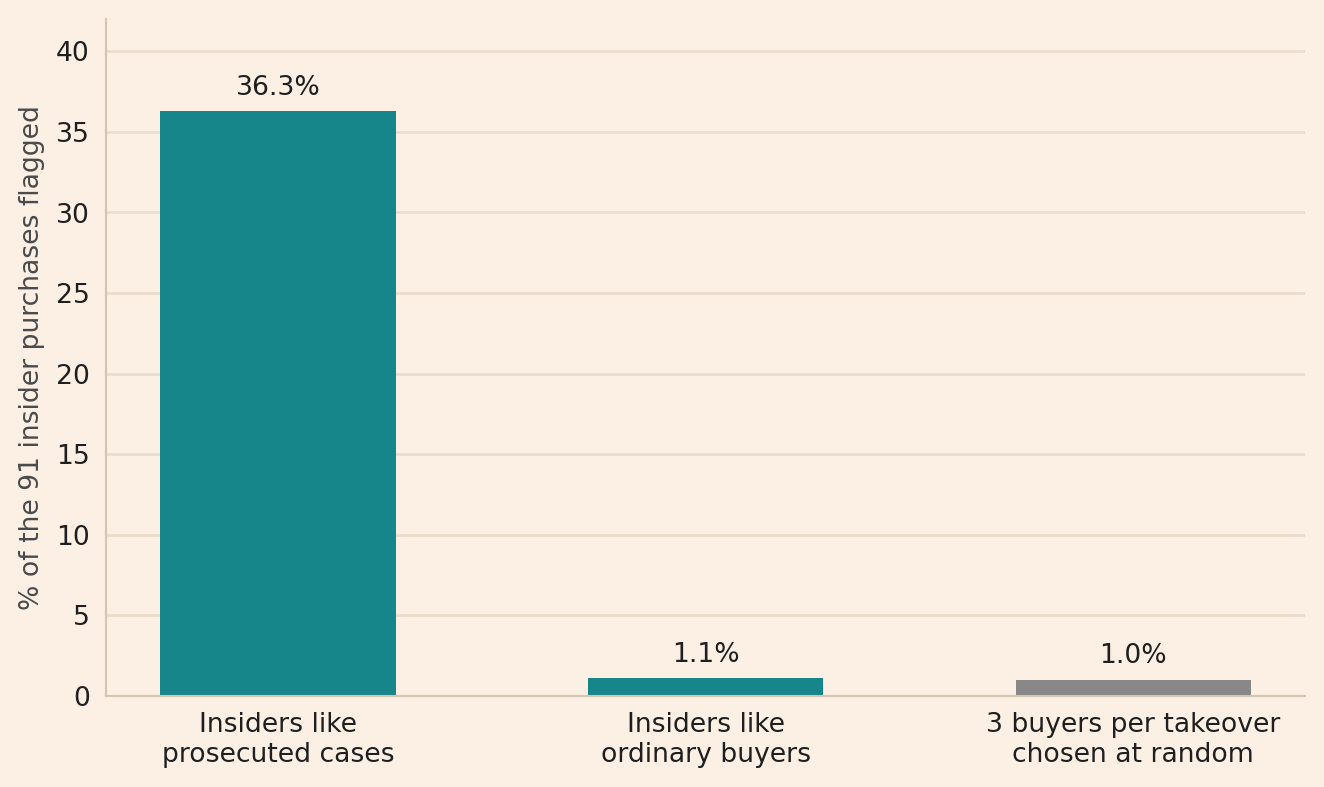

The teal bars are the forest’s shares of the 91 insider purchases flagged, 36.3% for insiders like prosecuted cases and 1.1% for insiders like ordinary buyers. The grey bar is the 1.0% that three buyers per takeover chosen at random would flag.

Limitations

A flag does not establish insider trading. 95.4% of the flags fall on ordinary buyers, and only evidence that a flagged buyer knew of the offer establishes insider trading.

Real insiders can be anywhere between the two versions. The first version resembles prosecuted cases, and the second buys like ordinary buyers.

The two parts are not one experiment. Part 1 counts stock-days and this post counts purchases, in different simulations, so the 6.4% there and the 36.3% here do not measure how much a broker’s records add.

One simulated broker. Every leak has insider accounts at this broker, the features are drawn independently of each other, and the forest is fitted on all 240 takeovers at once, after the fact. With real records the shares can differ.

Conclusion

In market data, the forest sees each stock-day, where a purchase of €50,000 may barely register in the day’s volume. A broker’s records show who bought, and an account in the target’s home city or a position ten times the client’s largest earlier one can make that same purchase stand out. In this simulation, the forest flags 36.3% of the purchases by insiders who trade like the prosecuted cases, almost all of them with a home-city link, and 1.1%, no better than chance, of the purchases by insiders who buy like ordinary buyers. The takeaway is that a broker’s records can reveal unusual purchases that a stock’s trading totals cannot, and the forest flags the insiders whose purchases are unusual in those records, not the ones who buy like everyone else.