import numpy as np
import pandas as pd

N_STOCKS = 2000
N_DAYS = 750
SEED = 2026                                    # fixed, so every number in the post reproduces
TAKEOVERS = 240                                # 4% of the stocks a year for three years
LEAKS = 48                                     # 1 in 5 takeovers, Patel and Putnins (2020)


def simulate_panel(seed):
    """Simulate the market as a panel with one row per stock-day and the columns ticker, date,
    return, volume and event. The event column is the answer key, used only to check alerts."""
    # rng is the random number generator, and the same seed, its starting number, always gives
    # the same draws.
    rng = np.random.default_rng(seed)

    # Ordinary trading. Draw each stock's base volatility, the scale of its daily log return
    # before the turbulence and the bounds below, and its base volume in shares a day.
    # rng.uniform(0.01, 0.03, N_STOCKS) draws one number per stock with equal chance anywhere
    # between 0.01 and 0.03.
    base_volatility = rng.uniform(0.01, 0.03, N_STOCKS)
    # 1e5 is 100,000 and 5e6 is 5 million. Drawing the base volume's logarithm with equal chance
    # anywhere between their logarithms makes a base volume of 100,000 to 1 million shares as
    # likely as one of 500,000 to 5 million.
    base_volume = np.exp(rng.uniform(np.log(1e5), np.log(5e6), N_STOCKS))

    # Two random factors that persist from one day to the next; each row is a day and each
    # column a stock. turbulence keeps 99% of the previous day's value, so a stock has calm and
    # turbulent periods that last months. activity keeps 60%, so a busy spell lasts only
    # days. A factor that keeps a share rho of its previous value and adds a normal draw with
    # standard deviation s has a long-run standard deviation of s / sqrt(1 - rho**2), where **
    # raises to a power. Day 0 is drawn with that standard deviation, so the stocks do not all
    # start from 0. np.zeros makes the 750-by-2,000 arrays that the loop fills in, and
    # rng.normal(0, s, N_STOCKS) draws one normal number per stock with a mean of 0 and a
    # standard deviation of s. range(1, N_DAYS) gives the days 1 to 749: it stops before 750.
    turbulence = np.zeros((N_DAYS, N_STOCKS))
    activity = np.zeros((N_DAYS, N_STOCKS))
    turbulence[0] = rng.normal(0, 0.05 / np.sqrt(1 - 0.99**2), N_STOCKS)
    activity[0] = rng.normal(0, 0.3 / np.sqrt(1 - 0.6**2), N_STOCKS)
    for day in range(1, N_DAYS):
        turbulence[day] = 0.99 * turbulence[day - 1] + rng.normal(0, 0.05, N_STOCKS)
        activity[day] = 0.6 * activity[day - 1] + rng.normal(0, 0.3, N_STOCKS)
    # base_volatility holds one value per stock, and NumPy multiplies each column of the
    # 750-by-2,000 array by its own stock's value.
    volatility = base_volatility * np.exp(turbulence)

    # The shock is the day's return in units of the stock's volatility. A Student t
    # distribution with 4 degrees of freedom gives very large draws more often than a normal
    # distribution, and dividing the draws by the square root of 2 gives them a standard
    # deviation of 1.
    shock = rng.standard_t(4, size=(N_DAYS, N_STOCKS)) / np.sqrt(2)
    # Each event multiplies volume by its own factor; 1 means no event on that stock-day.
    volume_multiplier = np.ones((N_DAYS, N_STOCKS))
    # The abnormal return that insider trading adds to a day's return; 0 on other stock-days.
    abnormal_return = np.zeros((N_DAYS, N_STOCKS))

    # Takeovers: 240 different target stocks. rng.choice(N_STOCKS, TAKEOVERS, replace=False)
    # draws 240 different stock numbers, and rng.integers(100, N_DAYS, TAKEOVERS) draws 240
    # whole numbers from 100 to 749, so the 40 days before each announcement have 60 earlier
    # days for the inputs. The first 48 leak: [True] * 48 is a list of 48 True values, and +
    # joins the lists. The price jump on each announcement day is 5% to 25%.
    takeovers = pd.DataFrame({
        "stock": rng.choice(N_STOCKS, TAKEOVERS, replace=False),
        "announcement_day": rng.integers(100, N_DAYS, TAKEOVERS),
        "leaked": [True] * LEAKS + [False] * (TAKEOVERS - LEAKS),
    })
    takeovers["announcement_return"] = rng.uniform(0.05, 0.25, TAKEOVERS)

    # Insider trading before each leaked announcement. The number of days is a geometric draw:
    # rng.geometric(1 / 3.2) counts the tries until a first success when each try succeeds
    # with probability 1 / 3.2, so it is at least 1, with a mean of 3.2 and a median of 2.
    # min(..., 40) keeps it within the 40 days available. The days are drawn from 1 to 40
    # trading days before the announcement: np.arange(1, 41) gives 1 to 40, stopping before
    # 41, and np.where gives each of the last 6 days a probability of 0.5 / 6 and each of the
    # 34 days before them 0.5 / 34, so each group has a chance of 1/2. rng.choice(...,
    # replace=False, p=weights) draws different days with those probabilities. On each day,
    # insider trading adds an abnormal return of 0% to 6% and multiplies volume by 1 to 2.86,
    # 3% and 1.93 on average.
    distances = np.arange(1, 41)
    weights = np.where(distances <= 6, 0.5 / 6, 0.5 / 34)
    insider_days = []                          # (days, stock) of each leak, for the event column
    # takeovers.loc[takeovers["leaked"]] keeps the rows where leaked is True, and itertuples()
    # hands them over one row at a time.
    for takeover in takeovers.loc[takeovers["leaked"]].itertuples():
        n_days = min(rng.geometric(1 / 3.2), 40)
        days = takeover.announcement_day - rng.choice(distances, n_days, replace=False, p=weights)
        abnormal_return[days, takeover.stock] = rng.uniform(0, 0.06, n_days)
        volume_multiplier[days, takeover.stock] = rng.uniform(1, 2.86, n_days)
        insider_days.append((days, takeover.stock))

    # News days and block trades: each stock-day has a 0.4% chance of each. rng.uniform draws a
    # number between 0 and 1 for each stock-day, which is below 0.004 with a probability of 0.4%.
    is_news_day = rng.uniform(size=(N_DAYS, N_STOCKS)) < 0.004
    is_block_trade = rng.uniform(size=(N_DAYS, N_STOCKS)) < 0.004
    # A stock-day drawn as both stays a news day. Indexing an array with is_news_day selects the
    # stock-days where is_news_day is True.
    is_block_trade[is_news_day] = False
    # No news day or block trade on a day of insider trading or an announcement day, so each of
    # those stock-days has one cause.
    for days, stock in insider_days:
        is_news_day[days, stock] = False
        is_block_trade[days, stock] = False
    for takeover in takeovers.itertuples():
        is_news_day[takeover.announcement_day, takeover.stock] = False
        is_block_trade[takeover.announcement_day, takeover.stock] = False

    # A news day replaces the shock with a move of 3 to 6 volatilities, up or down with equal
    # chance (rng.choice([-1, 1], ...) draws the sign), and multiplies volume by 1.5 to 3. A
    # block trade multiplies volume by 3 to 6. sum() counts the True entries, the number of
    # draws needed.
    n_news_days = is_news_day.sum()
    shock[is_news_day] = rng.choice([-1, 1], n_news_days) * rng.uniform(3, 6, n_news_days)
    volume_multiplier[is_news_day] = rng.uniform(1.5, 3, n_news_days)
    volume_multiplier[is_block_trade] = rng.uniform(3, 6, is_block_trade.sum())
    # 8 to 15 times the volume on each announcement day
    for takeover in takeovers.itertuples():
        volume_multiplier[takeover.announcement_day, takeover.stock] = rng.uniform(8, 15)

    # The shock times the volatility is the day's log return, the logarithm of the price ratio.
    # np.clip keeps it between -0.4 and 0.4, so the shock moves the price by -33% to
    # +49% at most in a day: a Student t shock inside the exponential would otherwise give
    # rare daily gains of more than 100%. np.exp gives the price ratio, above 0, so the ratio
    # minus 1, the return, stays above -100%; insider trading adds its abnormal return to it.
    log_return = np.clip(volatility * shock, -0.4, 0.4)
    returns = np.exp(log_return) - 1 + abnormal_return
    # Volume is higher in turbulent periods and busy spells, and on days with a large shock.
    # np.minimum(np.abs(shock), 10) caps the shock's part at 10, so one draw
    # multiplies volume by at most e^2, about 7.4. np.round(...).astype(int) gives whole shares.
    volume = np.round(base_volume * np.exp(0.5 * turbulence + activity
                                           + 0.2 * np.minimum(np.abs(shock), 10))
                      * volume_multiplier).astype(int)
    # On the announcement day the price jumps towards the offer price.
    for takeover in takeovers.itertuples():
        returns[takeover.announcement_day, takeover.stock] = takeover.announcement_return

    # The answer key: each stock-day's event, "no event" unless one of the events sets it.
    # dtype=object lets the array hold text.
    event = np.full((N_DAYS, N_STOCKS), "no event", dtype=object)
    event[is_news_day] = "news day"
    event[is_block_trade] = "block trade"
    for days, stock in insider_days:
        event[days, stock] = "insider trading"
    for takeover in takeovers.itertuples():
        event[takeover.announcement_day, takeover.stock] = "announcement day"

    # One row per stock-day, ordered by date, then ticker. ravel() turns a 750-by-2,000 array
    # into one long array, row by row: day 0 of every stock, then day 1, and so on. np.tile
    # repeats the 2,000 tickers once per day, and np.repeat repeats each date 2,000 times. In an
    # f-string, {number:04d} writes the number with four digits, 0007 for 7.
    tickers = [f"S{number:04d}" for number in range(N_STOCKS)]
    dates = pd.bdate_range("2023-01-02", periods=N_DAYS)    # 750 weekdays from 2 January 2023
    return pd.DataFrame({"ticker": np.tile(tickers, N_DAYS), "date": np.repeat(dates, N_STOCKS),
                         "return": returns.ravel(), "volume": volume.ravel(),
                         "event": event.ravel()})


panel = simulate_panel(SEED)Detecting unusual trading with an isolation forest, part 1: market data
Python
Machine Learning
Tutorial
Code
In a simulated market, an isolation forest flags only 6.4% of the days of insider trading, because most of those days look like ordinary days.
Exchanges and regulators look for illegal insider trading, called insider dealing in EU law: trading on inside information, such as a takeover offer that is not yet public. Say we look for it in market data, where each stock-day is one stock on one trading day. We can check only a few stock-days closely each day, and an isolation forest can choose which: it scores each stock-day by how unusual its return and volume are, without needing examples of past insider trading.
I test the forest on a simulated market in which the takeover offer leaks in 1 in 5 takeovers. On a few days before a leaked announcement, the days of insider trading, insiders buy shares of the target, the company being bought, which raises its return and volume as much as in prosecuted cases. Each day, the forest flags the 20 most unusual of the 2,000 stock-days. It flags 6.4% of the days of insider trading, and 98.2% of its alerts fall on stock-days unrelated to any takeover. A simpler rule, which flags the 20 stock-days with the highest volume relative to each stock’s usual volume, flags 12.2% of the days of insider trading. Both methods miss most of those days, because most of them look like many ordinary days.
This is part 1 of a pair and uses only what anyone with market data can see: each stock’s daily return and volume. Part 2 uses a broker’s records, which also show who traded, and asks which insider purchases an isolation forest flags there.
Simulating the data
I simulate 2,000 stocks over 750 trading days, three years, with one row per stock-day: ticker, date, return and volume. A fifth column, event, records what happened on the stock-day. Neither method sees the event column; I use it only to check which events each method’s alerts fall on. Besides ordinary trading, the market has four events:
- Insider trading. The offer leaks in 48 of 240 takeovers, 1 in 5, the share of mergers and acquisitions with insider trading that Patel and Putniņš (2020) estimate for US stocks. Insiders trade on 3.2 days per leak on average, and on each of those days the target’s return increases by 3 percentage points and its volume by 93% on average, as Meulbroek (1992) measures in cases prosecuted by the US Securities and Exchange Commission.
- Announcements. On the announcement day, the target’s price jumps by 5% to 25%, and its volume is 8 to 15 times its usual level. King (2009) reports average jumps of 6.4% to 21.4% in studies of US takeovers.
- News. On 0.4% of stock-days, public news moves the price up or down by 3 to 6 times the stock’s volatility, the typical size of its daily move, and increases volume.
- Block trades. On 0.4% of stock-days, a single large trade multiplies volume by 3 to 6.
The numbers without a source are assumptions. The box below gives the formulas and the code.
NoteHow the market is simulated
A stock’s return on day \(t\) is
\[r_t = e^{x_t} - 1 + \alpha_t, \qquad x_t = \min\big(\max(\sigma_t z_t,\, -0.4),\, 0.4\big), \qquad \sigma_t = \sigma\, e^{u_t}, \qquad u_t = 0.99\, u_{t-1} + \varepsilon_t ,\]
where \(x_t\) is the log return from ordinary trading, the logarithm of today’s price divided by yesterday’s, and \(\alpha_t\) is the abnormal return from insider trading, 0 on other days. The shock \(z_t\) is a draw from a Student t distribution with 4 degrees of freedom, divided by that distribution’s standard deviation, \(\sqrt{2}\), so it has a standard deviation of 1 and takes extreme values more often than a normal draw. The bounds of −0.4 and 0.4 keep the day’s move from ordinary trading between −33% and +49%, and the exponential, \(e\) raised to the log return, keeps the price ratio above 0, so the return stays above −100%. The volatility \(\sigma_t\) is the stock’s base volatility \(\sigma\), drawn with equal chance between 1% and 3%, times \(e^{u_t}\). The turbulence \(u_t\) keeps 99% of the previous day’s value and adds a normal draw \(\varepsilon_t\) with a standard deviation of 0.05, so calm and turbulent periods last months.
Volume is higher in turbulent periods, in busy spells and on days with a large shock in either direction:
\[v_t = V\, e^{\,0.5\, u_t + a_t + 0.2\, \min(|z_t|,\, 10)}\, m_t, \qquad a_t = 0.6\, a_{t-1} + \eta_t ,\]
where \(V\) is the stock’s base volume, between 100,000 and 5 million shares a day with each tenfold range equally likely. The activity \(a_t\) keeps 60% of the previous day’s value and adds a normal draw \(\eta_t\) with a standard deviation of 0.3, so a busy spell lasts days. Both \(u_t\) and \(a_t\) start from a draw with their long-run standard deviation. The cap of 10 on the shock limits its effect on volume to a factor of \(e^{2}\), about 7.4, and the event factor \(m_t\) is 1 unless an event multiplies volume. In the events, each range is drawn with every value equally likely:
- Takeovers. 240 different targets, each announced on a day drawn from the 101st on, so the 40 days before an announcement have 60 earlier days for the inputs below. That is 80 takeovers a year, close to the 75 a year that the UK’s Financial Conduct Authority counted over 2020 to 2023. On the announcement day, the return is 5% to 25% and \(m_t\) is 8 to 15.
- Leaks. The offer leaks in 48 of the takeovers. The number of days of insider trading is a geometric draw, in which 1 day is the most likely count and each extra day is less likely, with a mean of 3.2 and a median, the middle value, of 2. The days are drawn without repeats from the 40 trading days before the announcement, with half the chance spread over the last 6. So the median day of insider trading is 6 trading days before the announcement, as in Meulbroek’s cases. On each of those days, \(\alpha_t\) is 0% to 6% and \(m_t\) is 1 to 2.86, which average 3% and 1.93.
- News and block trades. Each stock-day has a 0.4% chance of news, which sets \(z_t\) to 3 to 6, up or down, and \(m_t\) to 1.5 to 3, and a 0.4% chance of a block trade, which sets \(m_t\) to 3 to 6. No stock-day has two events.
The block below simulates the panel.
Computing the two inputs
A 3% return is ordinary for a volatile stock and unusual for a calm one, so each input compares the stock-day with the same stock’s previous 60 trading days:
\[\text{standardised return}_t = \frac{r_t}{\hat\sigma_t}, \qquad \text{relative volume}_t = \frac{v_t}{\tilde v_t},\]
where the past volatility \(\hat\sigma_t\) is the standard deviation of the previous 60 returns and the past typical volume \(\tilde v_t\) is the median of the previous 60 volumes. The median, unlike the mean, changes little when one of those 60 days has an exceptional volume. The block below adds both inputs to the panel.
WINDOW = 60                                    # earlier trading days that each input uses


def past_volatility(returns):
    """One stock's standard deviation of its previous 60 returns, day by day. rolling(WINDOW)
    takes the 60 values ending at each row, and shift(1) first moves every value down one row,
    so the 60 days for day t end on day t - 1."""
    return returns.shift(1).rolling(WINDOW).std()


def past_typical_volume(volume):
    """One stock's median of its previous 60 volumes, day by day."""
    return volume.shift(1).rolling(WINDOW).median()


# groupby("ticker") hands each helper one stock's rows at a time, in date order, and
# transform() puts the results back in the panel's rows.
by_ticker = panel.groupby("ticker")
panel["standardised_return"] = panel["return"] / by_ticker["return"].transform(past_volatility)
panel["relative_volume"] = panel["volume"] / by_ticker["volume"].transform(past_typical_volume)

# The first 60 days of each stock have no inputs, and dropna() removes those rows. copy() makes
# stock_days a separate table, so pandas does not warn when columns are added to it.
stock_days = panel.dropna(subset=["standardised_return", "relative_volume"]).copy()
# An f-string, f"...", fills in the value of each expression in braces, and {x:,} writes x with
# commas between thousands.
print(f"stock-days with both inputs: {len(stock_days):,}\n")
columns = ["ticker", "date", "return", "volume", "standardised_return", "relative_volume"]
# stock_days.loc[rows, columns] keeps the rows where the condition is True, here S0000's, and
# the listed columns; head(3) keeps the first three rows.
first_rows = stock_days.loc[stock_days["ticker"] == "S0000", columns].head(3)
# round() with a dictionary rounds each named column to its own number of decimals
print(first_rows.round({"return": 4, "standardised_return": 2, "relative_volume": 2})
      .to_string(index=False))
stock-days with both inputs: 1,380,000
ticker date return volume standardised_return relative_volume
S0000 2023-03-27 0.0170 2211106 0.60 1.00
S0000 2023-03-28 0.0145 3243499 0.52 1.47
S0000 2023-03-29 0.0014 1774448 0.05 0.81Each stock’s first 60 days have no inputs, which leaves 690 of the 750 days per stock, 1,380,000 stock-days in all. On 27 March 2023, S0000’s return of 1.70% is 0.60 times its past volatility, and its volume equals its past typical volume, a relative volume of 1.00.
How an isolation forest works
An isolation forest splits the stock-days at random and measures how easily each one is isolated: the fewer random splits it takes to separate a stock-day from all the others, the more unusual the stock-day. Picture the stock-days as points, standardised return across and relative volume up. A split is a vertical or horizontal line at a random position. To isolate one stock-day, keep the points on its side of the line and split them again, until the stock-day is alone. A point far from the cloud of points is alone after a few splits, and a point inside the cloud needs many.
The forest does not split all 1,380,000 stock-days at once. It draws 256 stock-days at random, splits them until each is alone, and counts for every stock-day how many of those lines it takes to cut it off. It repeats this 100 times, with a new sample each time, and averages the counts. Each repetition is called a tree and the 100 together a forest. The 256 and the 100 are the defaults of scikit-learn, the Python library I use, and Liu, Ting and Zhou (2008), who proposed the method, found samples of 256 generally large enough. The average count, \(\bar h\), gives the isolation score:
\[\text{isolation score} = 2^{-\bar h / c(256)},\]
where \(c(256) = 10.24\) is the average number of splits needed to isolate one of 256 points. A stock-day that needs 10.24 splits on average scores 0.5, and a stock-day that needs fewer splits scores closer to 1. The score ranks the stock-days and is not a probability of insider trading.
Choosing twenty alerts a day
On each date, the forest’s alerts are the 20 stock-days with the highest isolation score, the top 1% of the date’s 2,000. So an alert is relative to its date: a score that misses the top 20 on a busy date can make it on a calm one. The 1% follows Cheng and co-authors (2023), who flag the 1% of client positions with the highest isolation scores at a large Chinese brokerage. For comparison, a volume-only rule flags the 20 stock-days with the highest relative volume on each date. I fit the forest on all three years at once, and a robustness check at the end fits it on a rolling one-year window instead.
from sklearn.ensemble import IsolationForest

INPUTS = ["standardised_return", "relative_volume"]
# scikit-learn's defaults repeat the random splitting 100 times (n_estimators=100), each time on
# 256 stock-days drawn at random (max_samples="auto"), so neither is written out. random_state
# fixes the random draws, so every run gives the same scores. contamination keeps its default
# too: it sets only the cut-off that predict() uses, and the scores do not depend on it.
forest = IsolationForest(random_state=SEED)
forest.fit(stock_days[INPUTS])                 # fit() draws the random splits from the stock-days
# score_samples() returns minus the isolation score, so a minus sign gives the score itself
stock_days["isolation_score"] = -forest.score_samples(stock_days[INPUTS])

ALERTS_PER_DAY = 20                            # stock-days flagged on each date


def top_each_day(column):
    """True for the ALERTS_PER_DAY stock-days with the highest value of column on each date.

    groupby("date") ranks each date's stock-days separately. rank(ascending=False) gives 1 to
    the highest value, and method="first" breaks ties by row order, so exactly 20 a day are
    marked.
    """
    rank = stock_days.groupby("date")[column].rank(ascending=False, method="first")
    return rank <= ALERTS_PER_DAY


stock_days["forest_alert"] = top_each_day("isolation_score")
stock_days["volume_alert"] = top_each_day("relative_volume")
# nunique() counts the different dates
print(f"alerts per method: {stock_days['forest_alert'].sum():,}, "
      f"20 on each of {stock_days['date'].nunique()} dates")
alerts per method: 13,800, 20 on each of 690 datesExamining the alerts
Over the 690 scored dates, each method gives 20 × 690 = 13,800 alerts. The block below compares each event’s share of the alerts with its share of all stock-days.
# value_counts(normalize=True) gives each event's share of the rows, and mul(100) turns the
# shares into percentages. stock_days.loc[rows, "event"] keeps the event column of the rows
# marked True, here each method's alerts.
EVENTS = ["insider trading", "announcement day", "news day", "block trade", "no event"]
shares = pd.DataFrame({
    "% of stock-days": stock_days["event"].value_counts(normalize=True),
    "% of forest alerts":
        stock_days.loc[stock_days["forest_alert"], "event"].value_counts(normalize=True),
    "% of volume-only alerts":
        stock_days.loc[stock_days["volume_alert"], "event"].value_counts(normalize=True),
}).reindex(EVENTS).fillna(0).mul(100)          # the rows in the order of EVENTS, 0 if absent
print(shares.round(3).to_string())
% of stock-days % of forest alerts % of volume-only alerts
event
insider trading 0.012 0.080 0.152
announcement day 0.017 1.739 1.725
news day 0.401 34.058 30.725
block trade 0.399 15.355 28.957
no event 99.170 48.768 38.442News days and block trades are each 0.4% of all stock-days, but they take 34.1% and 15.4% of the forest’s alerts. Days of insider trading are 0.012% of all stock-days and take 0.08% of the alerts, and announcement days take 1.7%. So 98.2% of the forest’s alerts, and 98.1% of the volume-only rule’s, fall on news days, block trades and stock-days made unusual by random variation.
Counting the flagged days of insider trading
What matters is the share of the days of insider trading that each method flags.
# The days of insider trading, and for each method the share of them with an alert, and the
# share of the leaks with an alert on at least one of their days. The mean of True and False
# values is the share of True. Each target has one takeover, so grouping the days of insider
# trading by ticker gives one row per leak, and any() is True where a leak has an alert.
insider_days = stock_days.loc[stock_days["event"] == "insider trading"]
methods = ["forest_alert", "volume_alert"]
flagged = pd.DataFrame({
    f"% of the {len(insider_days)} days of insider trading flagged":
        insider_days[methods].mean(),
    f"% of the {insider_days['ticker'].nunique()} leaks flagged":
        insider_days.groupby("ticker")[methods].any().mean(),
}).mul(100)
# rename() replaces the row names forest_alert and volume_alert with readable ones
flagged = flagged.rename(index={"forest_alert": "isolation forest",
                                "volume_alert": "volume-only rule"})
print(flagged.round(1).to_string())
% of the 172 days of insider trading flagged % of the 48 leaks flagged
isolation forest 6.4 22.9
volume-only rule 12.2 37.5The forest flags 6.4% of the 172 days of insider trading, and at least one day in 22.9% of the 48 leaked takeovers. The volume-only rule flags 12.2% of the days and at least one day in 37.5% of the leaks. Choosing 20 stock-days a day at random would flag 1% of the days. The chart below plots each method’s alerts among all stock-days, with the days of insider trading circled.
Show the chart code
import matplotlib.pyplot as plt

RED, TEAL, ORANGE, GREY = "#C0392B", "#17868A", "#D2822B", "#888888"
# The site's chart colours, in order: the cream background, the text, the light grid lines,
# the pale frame and the axis labels, the same on every chart of the site.
BG, INK, GRID, SPINE, AXIS_TEXT = "#FCEFE3", "#1f1f1f", "#EADCCC", "#D5C6B4", "#4a4a4a"


def style_chart(figure, axis):
    """Give a finished chart the site's cream background, light grid and pale frame."""
    figure.patch.set_facecolor(BG)
    axis.set_facecolor(BG)
    axis.grid(True, axis="y", color=GRID, lw=1.0)
    axis.set_axisbelow(True)
    for side in ("top", "right"):
        axis.spines[side].set_visible(False)
    for side in ("left", "bottom"):
        axis.spines[side].set_color(SPINE)
    axis.tick_params(axis="both", length=0, colors=INK, pad=6)
    axis.xaxis.label.set_color(AXIS_TEXT)
    axis.yaxis.label.set_color(AXIS_TEXT)
    axis.title.set_color(INK)
    # Write each legend entry in the colour of what it labels. get_legend() returns None when
    # the chart has no legend. hasattr() checks whether a handle has get_color().
    legend = axis.get_legend()
    if legend is not None:
        for text, handle in zip(legend.get_texts(), legend.legend_handles):
            if hasattr(handle, "get_color"):
                colour = handle.get_color()          # a line
            elif len(handle.get_facecolor()) > 0:   # an unfilled marker has no fill colours
                colour = handle.get_facecolor()      # a filled marker or a bar
            else:
                colour = handle.get_edgecolor()      # an unfilled marker takes its outline colour
            text.set_color(colour)


# Two charts side by side, one row of two, that share the vertical axis; axes[0] is the left
# chart. figsize is the figure's width and height in inches.
figure, axes = plt.subplots(1, 2, figsize=(11, 5), sharey=True)
for axis, alert_column, colour, title in [
        (axes[0], "forest_alert", TEAL, "Isolation forest alerts"),
        (axes[1], "volume_alert", ORANGE, "Volume-only alerts")]:
    alerted = stock_days.loc[stock_days[alert_column]]
    # rasterized=True stores the grey points as one image, which keeps the file small; s sets
    # the point size, and alpha=0.25 makes the points partly transparent
    axis.scatter(stock_days["standardised_return"], stock_days["relative_volume"], s=2,
                 color=GREY, alpha=0.25, rasterized=True)
    axis.scatter(alerted["standardised_return"], alerted["relative_volume"], s=6,
                 color=colour, label="alerts")
    # empty red circles, so the point inside each circle stays visible; lw is the circles' line
    # width
    axis.scatter(insider_days["standardised_return"], insider_days["relative_volume"], s=60,
                 facecolors="none", edgecolors=RED, lw=1.4, label="insider trading")
    axis.set_yscale("log")                  # each step up the axis multiplies the value by 10
    axis.set_xlim(-8, 8)
    axis.set_xlabel("Standardised return (return / past volatility)")
    axis.set_title(title)
    # the legend lists each label, without a box (frameon=False), in the top left corner
    axis.legend(frameon=False, loc="upper left")
    style_chart(figure, axis)
# the two charts share the vertical axis, so only the left one is labelled
axes[0].set_ylabel("Relative volume (volume / past typical volume, log scale)")
# tight_layout() fits the labels inside the figure. savefig writes the chart to a PNG file:
# dpi=140 sets its resolution, bbox_inches="tight" trims the empty margin, and facecolor=BG
# keeps the cream background. show() displays the chart.
plt.tight_layout()
plt.savefig("alerts_by_method.png", dpi=140, bbox_inches="tight", facecolor=BG)
plt.show()

# the stock-days beyond the horizontal axis's range of -8 to 8
beyond_chart = stock_days.loc[stock_days["standardised_return"].abs() > 8]
print(f"stock-days with a standardised return beyond 8 either way, left off the chart: "
      f"{len(beyond_chart)}, of which announcement days: "
      f"{(beyond_chart['event'] == 'announcement day').sum()}, "
      f"insider trading: {(beyond_chart['event'] == 'insider trading').sum()}")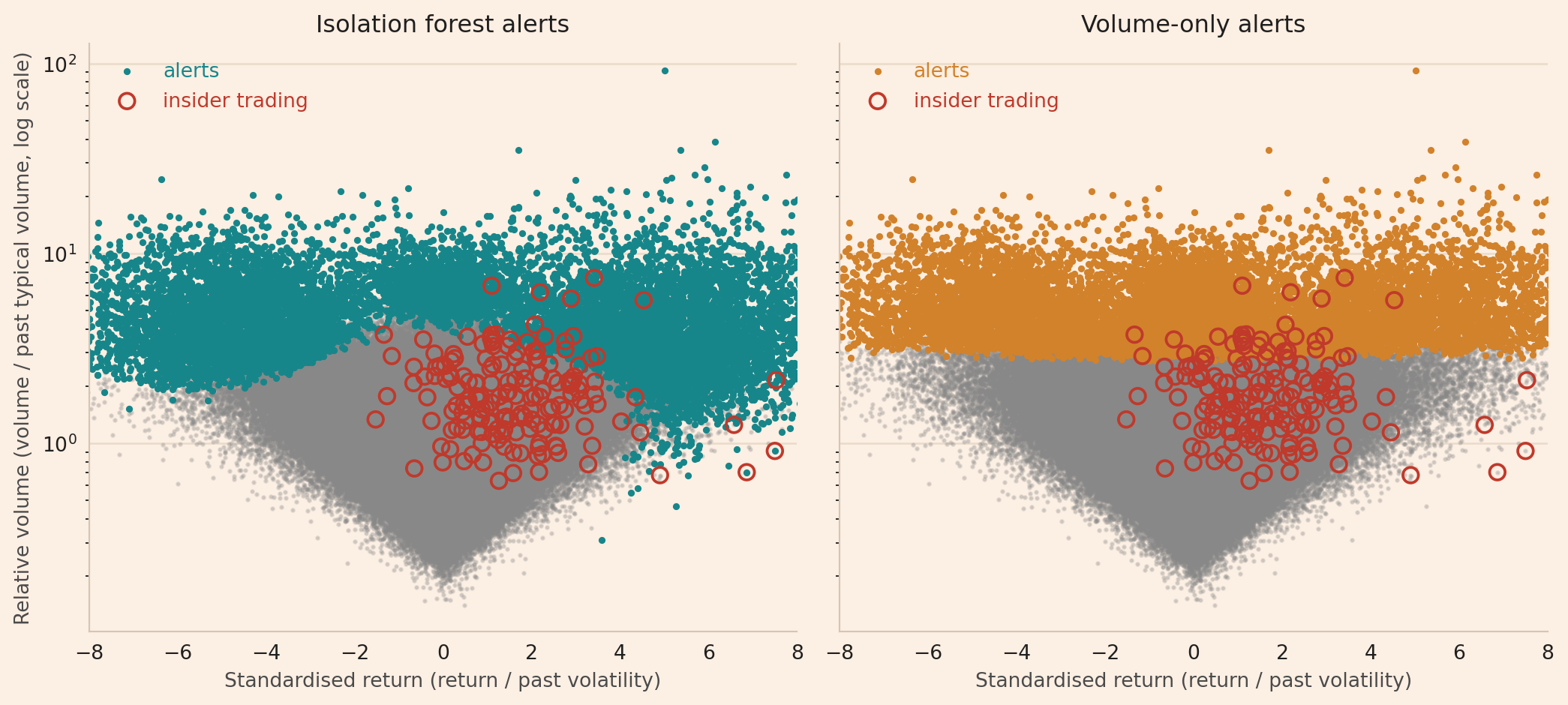
stock-days with a standardised return beyond 8 either way, left off the chart: 1054, of which announcement days: 104, insider trading: 0The red circles, the days of insider trading, are mostly inside the grey cloud of all stock-days. The forest’s teal alerts are at the cloud’s left and right edges, the largest price falls and rises, and at its top, the largest relative volumes. The volume-only rule’s orange alerts are at the top only. Most days of insider trading have an ordinary return, so the forest, which spends part of its alerts on large price moves, flags fewer of them than the volume-only rule. The vertical axis has a log scale, and 1,054 stock-days with a standardised return beyond −8 or 8 are left off the chart: 104 of them are announcement days, and none is a day of insider trading.
Why most insider trading is not flagged
The block below ranks each date’s 2,000 stock-days by isolation score and by relative volume, as percentiles, and looks at where the 172 days of insider trading fall. Only the top 1% of a date, above its 99th percentile, get alerts. The block prints the quartiles of the insider-trading days’ percentile ranks: the ranks that a quarter, half and three quarters of those days are below.
# rank(pct=True) turns the values of each date into percentiles: 1 is the date's highest value,
# and an alert needs one of the 20 highest of 2,000, a percentile above 0.99. quantile() gives
# the values below which a quarter, a half and three quarters of the days of insider trading
# fall, and mul(100) writes the percentiles on a scale of 0 to 100.
percentile = stock_days.groupby("date")[["isolation_score", "relative_volume"]].rank(pct=True)
insider_percentile = percentile.loc[stock_days["event"] == "insider trading"]
quartiles = insider_percentile.quantile([0.25, 0.5, 0.75]).mul(100)
quartiles.index = ["first quartile", "median", "third quartile"]
print(quartiles.round(1).to_string())
isolation_score relative_volume
first quartile 79.3 70.8
median 93.8 90.5
third quartile 97.8 97.5The quartiles of these percentile ranks are 79.3, 93.8 and 97.8 for the isolation score and 70.8, 90.5 and 97.5 for the relative volume. So three quarters of the days of insider trading rank below the 98th percentile of their date, short of the 99th that an alert needs. Insider trading lifts a stock-day’s return and volume, but on every date news days, block trades and random variation make other stock-days more unusual, and those take the 20 alerts. So most days of insider trading are disguised among ordinary days, although each moves return and volume as much as in prosecuted cases.
Robustness check: a rolling one-year window
As a robustness check, I fit the forest on a rolling one-year window, so that it uses only earlier data: every 20 dates, I refit it on the previous 250 dates and score the next 20. The first 250 dates have no year before them, so the check covers the last 440 dates, which hold 91 of the 172 days of insider trading. This forest and the forest fitted on all three years are each fitted five times, with random_state 2026 to 2030, because the forest’s random draws change a few alerts.
Show the code for the rolling one-year window
# Number the dates with inputs in time order, from 0. rank(method="dense") numbers the distinct
# dates 1, 2, 3 and so on, giving every stock-day of a date the same number, and - 1 starts at 0.
date_number = stock_days["date"].rank(method="dense").astype(int) - 1
EARLIER_DATES = 250                            # dates the splits are drawn from, about a year
DATES_PER_FOREST = 20                          # dates scored before new splits are drawn
scored = date_number >= EARLIER_DATES          # True from the 251st date on


def score_from_earlier_dates(seed):
    """Isolation scores from the 251st date on. Each forest draws its splits from the 250 dates
    before the first date it scores, so it uses no stock-day from the dates it scores
    or from later dates. The first 250 dates keep NaN, which marks a missing value."""
    # a Series with one missing value per stock-day, which the loop fills in, 20 dates at a time
    scores = pd.Series(np.nan, index=stock_days.index)
    # range(250, 690, 20) gives 250, 270 and so on up to 670: it steps by 20 and stops before
    # 690, the number of dates
    for first_scored in range(EARLIER_DATES, date_number.max() + 1, DATES_PER_FOREST):
        earlier_rows = ((date_number >= first_scored - EARLIER_DATES)
                        & (date_number < first_scored))
        scored_rows = ((date_number >= first_scored)
                       & (date_number < first_scored + DATES_PER_FOREST))
        # the same defaults as the forest above, with splits drawn from earlier stock-days only
        forest = IsolationForest(random_state=seed).fit(stock_days.loc[earlier_rows, INPUTS])
        # score_samples returns a NumPy array, which fills the selected rows in their order
        scores.loc[scored_rows] = -forest.score_samples(stock_days.loc[scored_rows, INPUTS])
    return scores


# The random draws also change a forest's alerts, so both kinds of forest run with five
# random_state values, 2026 to 2030. For each value, the loop counts the stock-days of insider
# trading from the 251st date on that each kind of forest flags. On the first 250 dates,
# score_earlier_days is NaN: rank() gives a missing score a missing rank, and a missing rank is
# not <= 20, so top_each_day flags none of those stock-days.
insider_scored = (stock_days["event"] == "insider trading") & scored
flagged = {}
for seed in range(SEED, SEED + 5):
    all_days_forest = IsolationForest(random_state=seed).fit(stock_days[INPUTS])
    stock_days["score_all_days"] = -all_days_forest.score_samples(stock_days[INPUTS])
    stock_days["score_earlier_days"] = score_from_earlier_dates(seed)
    flagged[seed] = {
        "forest fitted on all three years":
            (top_each_day("score_all_days") & insider_scored).sum(),
        "forest on a rolling one-year window":
            (top_each_day("score_earlier_days") & insider_scored).sum(),
    }
print(f"dates scored by both kinds of forest: {date_number.max() + 1 - EARLIER_DATES}, "
      f"with {insider_scored.sum()} stock-days of insider trading\n")
# pd.DataFrame(flagged) makes one column per random_state value and one row per kind of
# forest. Dividing each count by the stock-days of insider trading and multiplying by 100
# gives the percentage of them flagged, and rename_axis names the columns, so the header
# shows what each column is.
flagged_pct = pd.DataFrame(flagged) / insider_scored.sum() * 100
print("% of the stock-days of insider trading flagged")
print(flagged_pct.round(1).rename_axis(columns="random_state").to_string())
volume_pct = (stock_days["volume_alert"] & insider_scored).sum() / insider_scored.sum() * 100
print(f"\nvolume-only rule, the same for every random_state: {volume_pct:.1f}%")
dates scored by both kinds of forest: 440, with 91 stock-days of insider trading
% of the stock-days of insider trading flagged
random_state 2026 2027 2028 2029 2030
forest fitted on all three years 5.5 2.2 5.5 2.2 3.3
forest on a rolling one-year window 4.4 2.2 5.5 4.4 2.2
volume-only rule, the same for every random_state: 9.9%With the rolling window, the forest flags 2.2% to 5.5% of the 91 days of insider trading, depending on the random_state, the same range as the forest fitted on all three years. With 91 days, one day is 1.1 percentage points, so the runs differ by a few days. The volume-only rule has nothing to fit and no random draws, so it flags the same 9.9% in every run. The shares differ from the 6.4% and 12.2% over all dates because the 91 days are a subset of the 172. The window changes little because an alert compares only the stock-days of one date, and every simulated year follows the same rules. In a real market, a window that includes a crisis year could rank a date’s stock-days differently.
Limitations
The size of insider trading comes from prosecuted cases. Patel and Putniņš find that detection is more likely when trading is unusual. So insider trading that goes undetected may change return and volume less than in the prosecuted cases, and the forest and the volume-only rule would flag it less often.
One simulated market. The shares of the days of insider trading flagged hold for this simulation, with its assumptions for ordinary trading, news and block trades. With real data the shares can differ.
Conclusion
In this market, the most unusual stock-days are mostly news days, block trades and stock-days made unusual by random variation. A day of insider trading that moves return and volume as much as in prosecuted cases rarely reaches the top 1% of its date. The takeaway is that an outlier method flags insider trading only when the trading makes a stock-day unusual, so insider trading that leaves a stock-day looking ordinary, by design or because it is small, is hard to find this way.
Read next
- Detecting unusual trading with an isolation forest, part 2: broker records How an isolation forest on a broker’s records flags insiders who buy unlike the other clients.
- Estimating the frequency of market crimes What we can estimate about market crime when most crimes are never detected.
- Two models with 99% accuracy can rank an offender differently How to measure a model’s ranking once offenders are labelled.
Disclaimer: a teaching example on simulated data. The share of takeovers that leak and the size and timing of insider trading come from the studies cited below, and the other numbers are assumptions. Not investment advice.
Sources: scikit-learn, IsolationForest, for the method and the score formula. Fei Tony Liu, Kai Ming Ting and Zhi-Hua Zhou, Isolation Forest, IEEE International Conference on Data Mining (2008), for the sample of 256. Guang Cheng, Christian T. Lundblad, Zhishu Yang and Qi Zhang, Detecting Insider Trading in the Era of Big Data and Machine Learning, SSRN working paper, 2023 version (the link opens the latest version), for screening pooled trading with an isolation forest and flagging 1% of client positions. Lisa K. Meulbroek, An Empirical Analysis of Illegal Insider Trading, Journal of Finance (1992), for the number, timing and size of the days of insider trading. Vinay Patel and Tālis J. Putniņš, How Much Insider Trading Happens in Stock Markets?, SSRN working paper (2020), for the share of takeovers that leak. Michael R. King, Prebid Run-Ups Ahead of Canadian Takeovers: How Big Is the Problem?, Financial Management (2009), for the jump on the announcement day. Financial Conduct Authority, A revision of our market cleanliness statistic methodology, research note (2024), for the number of UK takeover announcements.