How active are active ETFs?
I am always curious to test whether something does what it is supposed to do. In the smart beta post, I tested whether smart beta ETFs are indeed smart compared with traditional ETFs. Here I want to test whether ETFs that are supposed to be active really are active.
Active means that the management of the ETF deviates, or tries to deviate, from its benchmark to outperform it, or to give an exposure that an investor could not get through passive investing. The benchmark is often explicit, but it does not have to be. This post measures how much the ETFs deviate from their benchmark. It does not test whether they outperformed it.
Measuring how active an ETF is
To measure how much an ETF deviates, I run an OLS regression with the ETF’s monthly return on the left-hand side and its benchmark’s monthly return on the right-hand side.
\[r_{\text{ETF},t} = \alpha + \beta\, r_{\text{benchmark},t} + \varepsilon_t\]
The R² then shows how much of the variation in the ETF’s return the variation in the benchmark can explain. It is 100% for an ETF that moves exactly with its benchmark.
\[R^2 = \operatorname{corr}\left(r_{\text{ETF}},\, r_{\text{benchmark}}\right)^2\]
The ETFs are US equity ETFs that traded every month from October 2023 to September 2026: 152 active and 263 index ETFs. Each ETF’s annual filing with the SEC says whether it is an index fund, and LSEG gives its benchmark. I have attached the code in the appendix.
Results
For 92% of the index ETFs, the R² is 99% or more, so almost all of their variation comes with the benchmark. For the active ETFs, the share is 4%. The median R² is 85.8% for the active ETFs and 99.95% for the index ETFs.
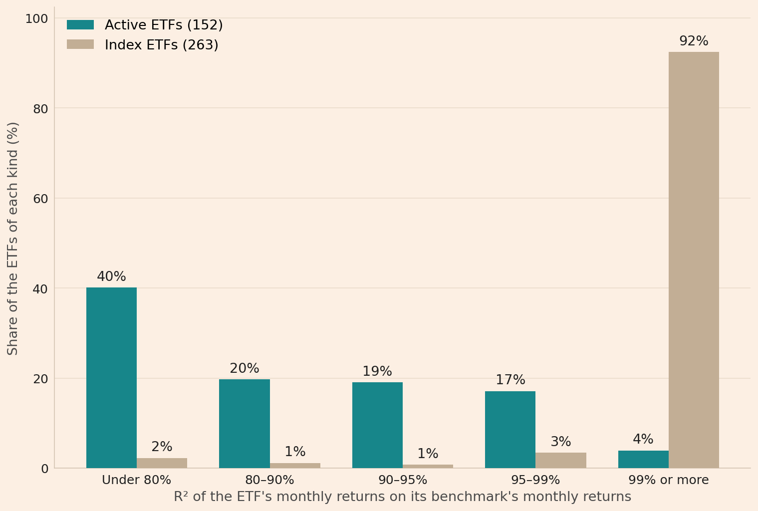
I also look at the tracking error to understand how much the ETF’s return varies around its benchmark’s return per year.
\[\text{tracking error} = \sigma\left(r_{\text{ETF},t} - r_{\text{benchmark},t}\right) \times \sqrt{12}\]
The median active ETF has a tracking error of 5.8 percentage points a year, and the median index ETF has 0.4.
So the active ETFs do move less closely with their benchmark than the index ETFs, but not by that much. The median active ETF has a tracking error of 5.8 points a year, while the median volatility of the active ETFs is 14.3% a year. And a few active ETFs behave almost like index ETFs. Six of the 152 have an R² of 99% or more.
Limitations
Some ETFs have no benchmark index in LSEG’s data, and some lack data in the sample period. Of the 805 US equity ETFs whose SEC filing says whether they are index funds, 248 (31%) have no benchmark index in LSEG’s data, and 142 (18%) lack some data in the period. So I only focus on the 415 ETFs that have a benchmark index, because I need it to see how active they are, and that have data in every month of the period, which is only three years.
When I fit each active ETF on four style indices at once (the S&P 500, the Russell 1000 Growth, the Russell 1000 Value, and the Russell 2000) instead of its own benchmark, the median R² is 90.2% instead of 85.8%, so the conclusion holds. R² and the tracking error measure how much the returns deviate. They do not measure how much the holdings deviate.
Conclusion
So the conclusion is that the active ETFs do move less closely with their benchmark than the index ETFs, but the difference is not that large. The median active ETF has a tracking error of 5.8 points a year.
Appendix: the code
# I start by loading the libraries in Python and naming the files that I will be working on. Then
# I specify the sample, and I also specify the five different R² bands and the four different
# style indices that I use when I do a sensitivity check for the ETFs. I specify everything that I
# will be reusing several times in the code, so that I do not need to specify it again.

import csv
import json
import warnings
import zipfile
from pathlib import Path

import matplotlib.pyplot as plt
import numpy as np
import pandas as pd
import statsmodels.api as sm

# Path.cwd() is the folder this notebook runs in, and / joins a folder and a file name
FOLDER = Path.cwd()
NCEN_FOLDER = FOLDER / "ncen"
UNIVERSE_FILE = FOLDER / "nr80_universe.csv"
REFERENCE_FILE = FOLDER / "nr80_reference.csv"
PRICES_FILE = FOLDER / "nr80_monthly_prices.csv"
DISTRIBUTIONS_FILE = FOLDER / "nr80_distributions.csv"
BENCHMARK_FILE = FOLDER / "nr80_benchmark_levels.csv"
NUMBERS_FILE = FOLDER / "active_etfs_numbers.json"
CHART_FILE = FOLDER / "active_etfs.png"

# The downloads run from August 2016 to September 2026, the last complete month, so that a window
# of up to ten years also has the month before its first month
START, END = "2016-08-01", "2026-09-30"
MONTHS = pd.period_range(START, END, freq="M")
# period_range with end= and periods= counts back from the last month, and END[:7] is 2026-09
YEARS = 3
WINDOW = pd.period_range(end=END[:7], periods=YEARS * 12, freq="M")
CHUNK = 25
# lseg-data 2.1.1 warns about pandas on every request, and filterwarnings turns that warning off
warnings.filterwarnings("ignore", category=FutureWarning, module="lseg")

# np.inf is infinity, so the last band holds an R² of exactly 100%
EDGES = [0, 80, 90, 95, 99, np.inf]
BANDS = ["Under 80%", "80–90%", "90–95%", "95–99%", "99% or more"]

STYLE_INDICES = ["S&P 500 TR", "Russell 1000 Growth TR", "Russell 1000 Value TR",
"Russell 2000 TR"]# Then I use LSEG to find US-based ETFs in the Lipper US equity classes and save them as a list,
# so that I only need to run the search once. I leave out the 357 that have closed, because almost
# all of them do not have enough data for the sample period I am interested in, and then I get 880
# ETFs that are still trading.
def open_lseg():
"""Opens the LSEG session, with LSEG Workspace running and logged in. The except branch fixes
an AttributeError of lseg-data 2.1.1 with httpx 0.28."""
import httpx
import lseg.data as ld
ld.get_config().set_param("http.request-timeout", 300)
try:
ld.open_session()
except AttributeError:
for client in (httpx.Client, httpx.AsyncClient):
original = client.__init__
def patched(self, *args, _original=original, **kwargs):
if isinstance(kwargs.get("proxy"), dict):
kwargs["proxy"] = next((value for value in kwargs["proxy"].values() if value),
None)
return _original(self, *args, **kwargs)
client.__init__ = patched
ld.open_session()
return ld
if not UNIVERSE_FILE.exists():
ld = open_lseg()
search_filter = ("IssuerDomicileCountryName eq 'United States'"
" and AssetCategoryName eq 'Fund Unit/Exchange Traded Fund'"
" and IsPrimaryRIC eq true"
" and startswith(IssueLipperGlobalSchemeName, 'Equity US')")
columns = "RIC,TickerSymbol,DTSubjectName,IssueLipperGlobalSchemeName"
found = ld.discovery.search(view=ld.discovery.Views.FUND_QUOTES, filter=search_filter,
select=columns, top=5000)
ld.close_session()
# top=5000 is the most rows one search returns, so fewer rows mean that the list is complete
assert len(found) < 5000, "the search stopped at its limit of 5,000 rows"
found.to_csv(UNIVERSE_FILE, index=False)
universe = pd.read_csv(UNIVERSE_FILE)
universe.columns = ["ric", "ticker", "name", "lipper_class"]
# LSEG marks a closed ETF's code with ^, such as TADS.K^A22, and ~ turns True into False
closed = universe["ric"].str.contains("^", regex=False)
trading = universe.loc[~closed]
# A ticker that two ETFs share cannot be matched with the SEC's files
shared_ticker = trading["ticker"].duplicated(keep=False)
trading = trading.loc[~shared_ticker]
print(f"US equity ETFs found: {len(universe)}")
print(f"Closed ETFs, left out: {closed.sum()}")
print(f"ETFs with a ticker that another ETF also has, left out: {shared_ticker.sum()}")
print(f"Trading ETFs: {len(trading)}")US equity ETFs found: 1237
Closed ETFs, left out: 357
ETFs with a ticker that another ETF also has, left out: 0
Trading ETFs: 880# Then I read the SEC's N-CEN filings to identify which of these are index ETFs. I only classify
# an ETF as index if it has filed as an index fund. The remaining ETFs I classify as active.
def read_table(archive, table, columns):
"""Reads one table of an N-CEN zip file, with only the columns asked for."""
for member in archive.namelist():
if Path(member).name.upper() == table + ".TSV":
with archive.open(member) as file:
return pd.read_csv(file, sep="\t", dtype=str, usecols=columns,
quoting=csv.QUOTE_NONE, encoding_errors="replace")
raise KeyError(f"no {table}.tsv in the zip file")
ncen_files = sorted(NCEN_FOLDER.glob("*.zip"))
assert len(ncen_files) > 0, f"no zip files in {NCEN_FOLDER}, so download the N-CEN data sets first"
tables = []
for path in ncen_files:
# with ... as closes the zip file at the end of the block
with zipfile.ZipFile(path) as archive:
submissions = read_table(archive, "SUBMISSION", ["ACCESSION_NUMBER", "FILING_DATE"])
answers = read_table(archive, "FUND_REPORTED_INFO",
["FUND_ID", "ACCESSION_NUMBER", "IS_INDEX", "IS_MULTI_INVERSE_INDEX"])
listings = read_table(archive, "SECURITY_EXCHANGE", ["FUND_ID", "FUND_TICKER_SYMBOL"])
# merge joins two tables on a column they share
tables.append(listings.merge(answers, on="FUND_ID").merge(submissions, on="ACCESSION_NUMBER"))
ncen = pd.concat(tables, ignore_index=True)
ncen = ncen.dropna(subset=["FUND_TICKER_SYMBOL"])
ncen["ticker"] = ncen["FUND_TICKER_SYMBOL"].str.strip().str.upper()
ncen["filed"] = pd.to_datetime(ncen["FILING_DATE"], format="mixed")
# Each ticker keeps its latest filing
ncen = ncen.sort_values("filed").drop_duplicates("ticker", keep="last")
# np.where(condition, a, b) gives a where the condition is True and b where it is False
ncen["kind"] = np.where(ncen["IS_INDEX"] == "Y", "index", "active")
ncen["leveraged"] = ncen["IS_MULTI_INVERSE_INDEX"] == "Y"
# how="left" keeps every trading ETF, with empty answers for a ticker without a filing
etfs = trading.merge(ncen[["ticker", "kind", "leveraged"]], on="ticker", how="left")
no_answer = etfs["kind"].isna()
# == True is False for an empty answer
leveraged = etfs["leveraged"] == True
labeled = etfs.loc[~no_answer & ~leveraged]
print(f"N-CEN files: {len(ncen_files)}")
print(f"Trading ETFs without an answer in the N-CEN files, left out: {no_answer.sum()}")
print(f"Leveraged or inverse ETFs, left out: {leveraged.sum()}")
print(f"ETFs labeled active or index: {len(labeled)}")
print(labeled["kind"].value_counts().to_string())N-CEN files: 8
Trading ETFs without an answer in the N-CEN files, left out: 71
Leveraged or inverse ETFs, left out: 4
ETFs labeled active or index: 805
kind
index 451
active 354# Then I download the benchmark of each ETF from LSEG, and I only include ETFs that have a
# benchmark index, because the purpose of this post is to compare each ETF with its benchmark. I
# need a benchmark in order to compute the R², and with a wrong benchmark, the R² becomes less
# accurate.
def download(codes, fields, parameters=None):
"""Downloads one LSEG table for a list of codes, CHUNK codes at a time."""
tables = []
for first in range(0, len(codes), CHUNK):
answer = ld.get_data(universe=codes[first:first + CHUNK], fields=fields,
parameters=parameters)
# The LSEG service can fail and give empty rows, and then the run stops before anything
# is saved
has_data = answer.drop(columns="Instrument").notna().any().any()
assert has_data, "LSEG gave no data for a request, so restart Workspace"
tables.append(answer)
return pd.concat(tables, ignore_index=True)
def is_saved(path, codes):
"""Returns True when the saved file at path lists every code."""
if not path.exists():
return False
return set(codes) <= set(pd.read_csv(path)["Instrument"])
rics = labeled["ric"].tolist()
if not is_saved(REFERENCE_FILE, rics):
ld = open_lseg()
download(rics, ["TR.FundBenchmarkName", "TR.FundBenchmarkInstrumentRIC"]
).to_csv(REFERENCE_FILE, index=False)
ld.close_session()
reference = pd.read_csv(REFERENCE_FILE).iloc[:, :3]
reference.columns = ["ric", "benchmark_name", "benchmark"]
assert reference["ric"].is_unique, "an ETF has more than one row of benchmark data"
# One benchmark code ends with an invisible space, and str.strip() removes it
reference["benchmark"] = reference["benchmark"].str.strip()
labeled = labeled.merge(reference, on="ric", how="left")
no_benchmark = labeled["benchmark"].isna()
with_benchmark = labeled.loc[~no_benchmark].copy()
print(f"ETFs without a benchmark index in LSEG's data, left out: {no_benchmark.sum()}")
print(f"ETFs with a benchmark index: {len(with_benchmark)}")ETFs without a benchmark index in LSEG's data, left out: 248
ETFs with a benchmark index: 557# Then I download the month-end prices and the distributions of the ETFs, and the month-end levels
# of their benchmarks, and save the results. I save all downloaded files, because otherwise it
# would take time every time I need to rerun the script after a change. So I only need to run the
# download once, and I can always reuse the sample data that I have downloaded.
# All the labeled ETFs, so that the notebook can count how many have the whole window
etf_codes = labeled["ric"].tolist()
benchmark_codes = with_benchmark["benchmark"].unique().tolist()
need_prices = not is_saved(PRICES_FILE, etf_codes)
need_distributions = not is_saved(DISTRIBUTIONS_FILE, etf_codes)
need_levels = not is_saved(BENCHMARK_FILE, benchmark_codes)
if need_prices or need_distributions or need_levels:
ld = open_lseg()
# Frq "M" gives the last closing price, or index level, of each month
month_end = {"SDate": START, "EDate": END, "Frq": "M"}
if need_prices:
download(etf_codes, ["TR.ClosePrice.date", "TR.ClosePrice"], month_end
).to_csv(PRICES_FILE, index=False)
if need_distributions:
# The dates do not select by ex-dividend date, so the window is wide
download(etf_codes, ["TR.DivExDate", "TR.DivAdjustedGross"],
{"SDate": START, "EDate": "2026-12-31"}).to_csv(DISTRIBUTIONS_FILE, index=False)
if need_levels:
download(benchmark_codes, ["TR.ClosePrice.date", "TR.ClosePrice"], month_end
).to_csv(BENCHMARK_FILE, index=False)
ld.close_session()
print("The prices, distributions, and benchmark levels are saved")The prices, distributions, and benchmark levels are saved# Then I compute the monthly returns of the ETFs, including the distributions, and the monthly
# returns of their benchmarks.
def month_end_table(path, codes):
"""Reads a saved LSEG file as one row per month and one column per code."""
values = pd.read_csv(path)
values.columns = ["ric", "date", "value"]
values = values.dropna()
# to_period("M") turns each date into its month, such as 2023-10
values["month"] = pd.to_datetime(values["date"].str[:10]).dt.to_period("M")
values = values.loc[values["month"].isin(MONTHS)]
# Each code keeps the last value of each month
values = values.sort_values("date").drop_duplicates(["ric", "month"], keep="last")
table = values.pivot(index="month", columns="ric", values="value")
return table.reindex(index=MONTHS, columns=codes)
month_end_price = month_end_table(PRICES_FILE, etf_codes)
benchmark_level = month_end_table(BENCHMARK_FILE, benchmark_codes)
distributions = pd.read_csv(DISTRIBUTIONS_FILE)
distributions.columns = ["ric", "ex_date", "amount"]
# Most rows without an amount are distributions announced for after September 2026. The few in
# the window count as no payment, and the notebook prints how many there are
ex_month = pd.to_datetime(distributions["ex_date"].str[:10]).dt.to_period("M")
no_amount = distributions["amount"].isna() & ex_month.isin(WINDOW)
distributions = distributions.dropna()
distributions["month"] = pd.to_datetime(distributions["ex_date"].str[:10]).dt.to_period("M")
distributions = distributions.loc[distributions["month"].isin(MONTHS)]
# A payment listed twice counts once
repeated = distributions.duplicated(["ric", "ex_date", "amount"])
distributions = distributions.loc[~repeated]
# fillna(0) says that a month without an ex-dividend date paid nothing
paid = distributions.pivot_table(index="month", columns="ric", values="amount", aggfunc="sum")
paid = paid.reindex(index=month_end_price.index, columns=month_end_price.columns).fillna(0)
# shift(1) takes the price at the end of the month before. A distribution is added at the end of
# its month, without reinvestment within the month
price_before = month_end_price.shift(1)
monthly = (month_end_price + paid) / price_before - 1
benchmark_monthly = benchmark_level / benchmark_level.shift(1) - 1
# An unchanged price may be stale, so such months are counted
stale = (month_end_price.loc[WINDOW] == price_before.loc[WINDOW]).sum().sum()
print(f"Distributions listed twice, counted once: {repeated.sum()}")
print(f"Distributions in the window without an amount, counted as no payment: {no_amount.sum()}")
print(f"ETFs with prices: {month_end_price.notna().any().sum()} of {len(etf_codes)}")
print(f"Benchmarks with levels: {benchmark_level.notna().any().sum()} of {len(benchmark_codes)}")
print(f"Months in the window with a price equal to the month before: {stale}")Distributions listed twice, counted once: 1
Distributions in the window without an amount, counted as no payment: 8
ETFs with prices: 793 of 805
Benchmarks with levels: 274 of 345
Months in the window with a price equal to the month before: 16# Then I compare each ETF with its benchmark over the sample period, only including those that
# have available data in every month. I compute the R², the tracking error, and the volatility. As
# a check, I use two ETFs, VOO and IVV, because they should be highly correlated with their
# benchmark and have a low tracking error, since they have filed as index funds.
rows = []
# The kind of each ETF that misses a month, and of each ETF whose benchmark misses one
etf_gap = []
benchmark_gap = []
large_moves = []
# iterrows() gives each row of the table with its label, and etf["ric"] is the row's code
for index, etf in with_benchmark.iterrows():
pair = pd.DataFrame({"etf": monthly.loc[WINDOW, etf["ric"]],
"benchmark": benchmark_monthly.loc[WINDOW, etf["benchmark"]]})
# all() asks whether every month is present, and continue goes on to the next ETF
if not pair["etf"].notna().all():
etf_gap.append(etf["kind"])
continue
if not pair["benchmark"].notna().all():
benchmark_gap.append(etf["kind"])
continue
# A split that the prices are not adjusted for would show as a move of 50% or more
if pair["etf"].abs().max() >= 0.5:
large_moves.append(etf["ticker"])
continue
# The R² is the squared correlation, in %, and ** raises to a power
r_squared = pair["etf"].corr(pair["benchmark"]) ** 2 * 100
# √12 turns a monthly standard deviation into a yearly one
difference = pair["etf"] - pair["benchmark"]
rows.append({"ric": etf["ric"], "ticker": etf["ticker"], "kind": etf["kind"],
"benchmark_name": etf["benchmark_name"], "r_squared": r_squared,
"tracking_error": difference.std() * np.sqrt(12) * 100,
"volatility": pair["etf"].std() * np.sqrt(12) * 100,
"benchmark_volatility": pair["benchmark"].std() * np.sqrt(12) * 100})
compared = pd.DataFrame(rows)
print(f"ETFs compared from {WINDOW[0]} to {WINDOW[-1]}: {len(compared)}")
print(f"ETFs with a monthly move of 50% or more, left out: {len(large_moves)} "
+ ", ".join(large_moves))
print("ETFs left out because a month of the ETF is missing, by kind:",
pd.Series(etf_gap, dtype=str).value_counts().to_dict())
print("ETFs left out because a month of the benchmark is missing, by kind:",
pd.Series(benchmark_gap, dtype=str).value_counts().to_dict())
# The ETFs' returns include distributions, so each benchmark should too. Its name says so with
# TR, NR, Total Return or Gross
total_return = compared["benchmark_name"].str.contains(r"\bTR\b|\bNR\b|Total Return|Gross")
print("ETFs whose benchmark is named as a total or net return index, by kind:",
compared.loc[total_return, "kind"].value_counts().to_dict())
# Month-end distributions and closing prices that differ from the net asset value can give even
# VOO and IVV a few tenths of a point
check = compared.loc[compared["ticker"].isin(["VOO", "IVV"])]
passed = ((check["r_squared"] >= 99.9) & (check["tracking_error"] < 0.5)).sum()
print(f"VOO and IVV with an R² of 99.9% or more and a tracking error under 0.5 percentage points "
f"a year: {passed} of {len(check)}")ETFs compared from 2023-10 to 2026-09: 415
ETFs with a monthly move of 50% or more, left out: 0
ETFs left out because a month of the ETF is missing, by kind: {'active': 36, 'index': 22}
ETFs left out because a month of the benchmark is missing, by kind: {'index': 74, 'active': 10}
ETFs whose benchmark is named as a total or net return index, by kind: {'index': 242, 'active': 152}
VOO and IVV with an R² of 99.9% or more and a tracking error under 0.5 percentage points a year: 2 of 2# Then I place each ETF into one of these R² bands, and I count the share of active and index ETFs
# in each band. I compute the median R², tracking error, and volatility of the active and of the
# index ETFs. I use the median to avoid the results being influenced by outliers, as they would be
# with the mean.
# right=False puts an R² of exactly 95% into "95–99%"
compared["band"] = pd.cut(compared["r_squared"], EDGES, labels=BANDS, right=False)
# crosstab counts the ETFs of each kind (the columns) in each band (the rows)
counts = pd.crosstab(compared["band"], compared["kind"]).reindex(BANDS, fill_value=0)
# Dividing by counts.sum() gives each band's share of its kind
shares = counts / counts.sum() * 100
print("ETFs in each R² band:")
print(counts.to_string())
print("\nShare of each kind in each R² band (%):")
print(shares.round(1).to_string())
medians = compared.groupby("kind")[["r_squared", "tracking_error", "volatility",
"benchmark_volatility"]].median()
print("\nMedians by kind (R² in %, tracking error in percentage points a year, volatilities in % "
"a year):")
print(medians.round(2).to_string())
# The median tracking error of all the ETFs in each band, active and index together, because some
# bands hold only two or three index ETFs
band_tracking_error = compared.groupby("band", observed=True)["tracking_error"].median()
print("\nMedian tracking error of the ETFs in each R² band (percentage points a year):")
print(band_tracking_error.reindex(BANDS).round(2).to_string())ETFs in each R² band:
kind active index
band
Under 80% 61 6
80–90% 30 3
90–95% 29 2
95–99% 26 9
99% or more 6 243
Share of each kind in each R² band (%):
kind active index
band
Under 80% 40.1 2.3
80–90% 19.7 1.1
90–95% 19.1 0.8
95–99% 17.1 3.4
99% or more 3.9 92.4
Medians by kind (R² in %, tracking error in percentage points a year, volatilities in % a year):
r_squared tracking_error volatility benchmark_volatility
kind
active 85.81 5.82 14.28 12.42
index 99.95 0.36 14.37 14.27
Median tracking error of the ETFs in each R² band (percentage points a year):
band
Under 80% 9.79
80–90% 5.54
90–95% 3.98
95–99% 2.52
99% or more 0.35# Then I do a final sensitivity check with the four style indices, to check how the R² changes
# when I use them as the benchmark instead.
style_codes = []
for name in STYLE_INDICES:
found = with_benchmark.loc[with_benchmark["benchmark_name"] == name, "benchmark"].unique()
assert len(found) == 1, f"{name} has more or fewer than one code"
style_codes.append(found[0])
style_returns = benchmark_monthly.loc[WINDOW, style_codes]
assert style_returns.notna().all().all(), "a style index misses a month of the window"
# add_constant adds the regression's constant
explain = sm.add_constant(style_returns)
style_r_squared = []
for ric in compared["ric"]:
# rsquared is the share of the variation that the four indices explain
fit = sm.OLS(monthly.loc[WINDOW, ric], explain).fit()
style_r_squared.append(fit.rsquared * 100)
compared["style_r_squared"] = style_r_squared
print("Median R² on the benchmark and on the four style indices (%):")
print(compared.groupby("kind")[["r_squared", "style_r_squared"]].median().round(2).to_string())Median R² on the benchmark and on the four style indices (%):
r_squared style_r_squared
kind
active 85.81 90.19
index 99.95 93.25# Then I save the results for the charts to use.
# {kind: ... for kind in KINDS} makes one entry for each kind
KINDS = ["active", "index"]
style_medians = compared.groupby("kind")["style_r_squared"].median()
numbers = {
"window": [str(WINDOW[0]), str(WINDOW[-1])],
"labeled": len(labeled),
"no_benchmark": int(no_benchmark.sum()),
"missing_month": len(etf_gap) + len(benchmark_gap),
"compared": {kind: int((compared["kind"] == kind).sum()) for kind in KINDS},
"bands": BANDS,
"counts": {kind: [int(count) for count in counts[kind]] for kind in KINDS},
"shares": {kind: [float(share) for share in shares[kind]] for kind in KINDS},
"medians": {column: {kind: float(medians.loc[kind, column]) for kind in KINDS}
for column in medians.columns},
"style_median_r_squared": {kind: float(style_medians[kind]) for kind in KINDS},
"band_tracking_error": [float(value) for value in band_tracking_error.reindex(BANDS)],
}
NUMBERS_FILE.write_text(json.dumps(numbers, indent=2), encoding="utf-8")
print(f"The numbers are saved in {NUMBERS_FILE.name}")The numbers are saved in active_etfs_numbers.json# Then I show the share of active and index ETFs in each of the R² bands as bars, in my site's
# colors, and save the chart.
# The site's chart colors
BG, INK, GRID, SPINE, AXIS_TEXT = "#FCEFE3", "#1f1f1f", "#EADCCC", "#D5C6B4", "#4a4a4a"
TEAL, SAND = "#17868A", "#C2AE95"
WIDTH = 0.38
# Each kind's bar is drawn half a bar's width to the left or the right of its band
positions = np.arange(len(BANDS))
figure, axis = plt.subplots(figsize=(12, 8))
for kind, offset, color, label in [
("active", -WIDTH / 2, TEAL, f"Active ETFs ({numbers['compared']['active']})"),
("index", WIDTH / 2, SAND, f"Index ETFs ({numbers['compared']['index']})")]:
bars = axis.bar(positions + offset, shares[kind], WIDTH, color=color, label=label, zorder=3)
# %.0f%% writes each bar's value as a whole percentage
axis.bar_label(bars, fmt="%.0f%%", padding=4, fontsize=13, color=INK)
axis.set_xticks(positions, BANDS)
axis.set_xlabel("R² of the ETF's monthly returns on its benchmark's monthly returns", fontsize=13,
color=AXIS_TEXT)
axis.set_ylabel("Share of the ETFs of each kind (%)", fontsize=13, color=AXIS_TEXT)
axis.set_ylim(0, shares.max().max() + 10)
axis.legend(frameon=False, fontsize=13)
figure.patch.set_facecolor(BG)
axis.set_facecolor(BG)
axis.grid(True, axis="y", color=GRID)
axis.set_axisbelow(True)
axis.spines[["top", "right"]].set_visible(False)
axis.spines[["left", "bottom"]].set_color(SPINE)
axis.tick_params(axis="both", length=0, colors=INK, pad=6, labelsize=12)
# The chart is saved at 150 dots per inch, and show() draws it below
plt.savefig(CHART_FILE, dpi=150, bbox_inches="tight", facecolor=BG)
plt.show()Read next
- How smart are smart beta ETFs? From November 2015 to September 2026, the ETFs of all seven smart beta strategies had a lower average Sharpe ratio than their cap-weighted benchmarks.
- Do income ETFs pay off? Only 4 of 96 US income ETFs had a higher annual return than SPY over the same months.
- How do ETFs work? Creation and redemption, step by step Why the price of an ETF’s shares stays close to the value of the ETF’s stocks.
Disclaimer: an empirical study for discussion purposes, not investment advice. The design is descriptive and not causal. Past performance does not guarantee future returns.
Data: the list of ETFs, their benchmarks, month-end closing prices and distributions, and the benchmarks’ month-end levels from LSEG Workspace (licensed). I do not reproduce the raw data here. Each fund’s answer to item C.3 of Form N-CEN from the SEC’s N-CEN data sets. The dots in the chart with steps are simulated: 36 months with the medians’ R² and tracking error.