How smart are smart beta ETFs?
The S&P 500 is cap-weighted: it weights its companies by the market value of their shares available to the public, so the largest companies get the largest weights. An exchange-traded fund (ETF) that tracks the index aims to earn the index’s return, less the fund’s fees. Smart beta ETFs choose and weight companies by a rule meant to improve on cap weighting, by earning more than a cap-weighted index or by earning as much with less risk. So the question is whether a smart beta fund did better than the cap-weighted index fund it could replace.
The rules differ by strategy. Value funds favour stocks with low prices relative to their earnings or book value, quality funds profitable companies, and momentum funds the stocks that rose the most over the past year. Low-volatility funds favour stocks whose prices move less, and dividend funds high and growing dividends. Multi-factor funds combine several rules, and equal-weight funds give every company the same weight.
I measure whether a rule improved on the index in two ways. The first is the return. The second is the Sharpe ratio, the average return above cash per unit of volatility, where volatility measures how much the returns vary. A rule that aims at less risk, such as low volatility, can earn less than the index and still have a higher Sharpe ratio.
I compare 21 selected US smart beta ETFs, three in each of the seven strategies, with their cap-weighted benchmarks from November 2015 to September 2026. On average, only the momentum funds earned more than their benchmarks, 0.93 percentage points a year. In all seven strategies, the funds’ average Sharpe ratio was lower than their benchmarks’, by 0.01 for quality up to 0.24 for value and equal weight. So, in return per unit of risk, no strategy improved on cap weighting on average over this period.
The test
Each fund is compared with a cap-weighted benchmark over the same months.
- Funds. Three ETFs in each of the seven strategies, 21 in all, that hold large US companies. I selected them among the largest by assets, all trading by October 2015 and still trading today, and have not checked their sizes against a dated list. DGRW, one of the quality funds, selects dividend payers by quality and growth, so it is also a dividend fund.
- Scope. The test covers funds that select or weight companies by a rule other than market value. So it leaves out the growth and value funds that weight their companies by market value. It also leaves out funds that weight companies by sales, earnings or book value, because those funds, like the value funds, give more weight to companies with low prices relative to these numbers.
- Benchmarks. Each fund is compared with one of five cap-weighted benchmarks: the S&P 500, MSCI USA, the Russell 1000, the whole US market or the Nasdaq-100. For 12 funds, the benchmark is the index from which the fund’s own index selects its companies. For the other 9, the fund’s own index selects from another list of companies, so the benchmark is the most similar of the five. As a check, I also compare every fund with SPY.
- Benchmark returns. For MSCI USA, I use the index itself, with dividends reinvested and no fees. For the other four, I use the ETFs that track them, SPY, IWB, VTI and QQQ, so their returns are after the ETFs’ fees.
- Returns. Monthly total returns, the price change plus reinvested dividends, after the funds’ fees, over 131 months. The months run from November 2015, the first full month after the youngest fund, SPMO, started trading, to September 2026. Each fund’s returns include any change of its index during the period.
Starting point
The comparison needs the monthly returns of the funds and their benchmarks, and a cash rate. The returns of the ETFs and the levels of MSCI USA come from LSEG Workspace, and the 3-month Treasury bill rate from FRED, the database of the Federal Reserve Bank of St. Louis. Because the LSEG data is licensed, I show the code without running it here, with the output of my run, and the output gives results only as averages by strategy or counts across funds.
Each calculation’s code is in an expandable block beside its explanation. It runs after the code in the appendix, which downloads the data, chooses one LSEG code per ETF and builds the monthly returns.
Step 1. Return and risk
To see whether a fund improved on its benchmark, I first measure both in the same way over the same 131 months, by their annual return and by their return per unit of risk. The annual return is
\[R = \left(\prod_{m=1}^{N} (1 + r_m)\right)^{12/N} - 1,\]
where \(r_m\) is the total return in month \(m\), as a decimal, and \(N = 131\) is the number of months. The product is what one dollar invested at the start of November 2015 was worth at the end of September 2026. The power \(12/N\) turns that growth into the yearly rate that gives the same growth.
The Sharpe ratio divides the average monthly return above cash by the standard deviation of that return, and makes the result annual:
\[S = \sqrt{12}\;\frac{\operatorname{mean}(r_m - c_m)}{\operatorname{sd}(r_m - c_m)},\]
where \(c_m\) is the cash return in month \(m\). The standard deviation, \(\operatorname{sd}\), measures how far the monthly values typically are from their average.
For \(c_m\), I take the 3-month Treasury bill rate at the end of the month before and divide it by 12. A Treasury bill is short-term US government debt, and \(c_m\) approximates what a bill bought at the end of the month before earned in month \(m\).
Multiplying by \(\sqrt{12}\) assumes that the monthly returns above cash are independent of each other, with the same average and standard deviation every month. Their sum over 12 months then has 12 times the monthly average and \(\sqrt{12}\) times the monthly standard deviation, because the variances, the squared standard deviations, add up. Dividing the two gives the factor \(\sqrt{12}\).
The volatility, the standard deviation of the monthly returns made annual in the same way, shows how much each series’ returns varied:
\[\sigma = \sqrt{12}\,\operatorname{sd}(r_m).\]
# One row per series: the annual return and the volatility in %, and the Sharpe ratio
measures = pd.DataFrame({
    "annual return": ((1 + monthly).prod() ** (12 / len(monthly)) - 1) * 100,
    "volatility": monthly.std() * np.sqrt(12) * 100,
    "Sharpe ratio": excess.mean() / excess.std() * np.sqrt(12)})
The block computes the three measures for each of the 26 series. Step 2 prints them as differences from the benchmarks, averaged by strategy.
Step 2. Differences from the benchmarks
A fund improved on its benchmark in a measure when the fund’s value is the higher one. So, for each fund \(i\), I subtract its benchmark’s annual return and Sharpe ratio:
\[\Delta R_i = R_i - R_{b(i)}, \qquad \Delta S_i = S_i - S_{b(i)},\]
where \(b(i)\) is the benchmark of fund \(i\). The difference in volatility is computed the same way.
Then I average the three funds’ differences within each strategy \(g\):
\[\overline{\Delta R}_g = \frac{1}{3}\sum_{i \in g} \Delta R_i, \qquad \overline{\Delta S}_g = \frac{1}{3}\sum_{i \in g} \Delta S_i,\]
which gives each fund the same weight. The average is not the difference of a portfolio that holds the three funds, because that portfolio’s Sharpe ratio also depends on how the funds’ returns vary together.
# Each fund's row minus its benchmark's row. map replaces each fund's benchmark with the name
# of its series, and set_axis names the benchmark rows after the funds, so the subtraction
# pairs each fund with its benchmark
benchmark_of = pd.Series(BENCHMARK).map(BENCHMARK_SERIES)
fund_rows = measures.loc[benchmark_of.index]
benchmark_rows = measures.loc[benchmark_of].set_axis(benchmark_of.index)
differences = fund_rows - benchmark_rows
differences["strategy"] = differences.index.map(STRATEGY)
strategies = differences.groupby("strategy").mean()
# Each comparison gives True or False for each fund, and sum() counts the True values
higher_sharpe = differences["Sharpe ratio"] > 0
higher_both = higher_sharpe & (differences["annual return"] > 0)
# The check: each fund's row minus SPY's row
differences_spy = fund_rows - measures.loc["SPY"]
differences_spy["strategy"] = differences_spy.index.map(STRATEGY)

print("Average of the three funds' differences from their benchmarks")
print("(annual return and volatility in percentage points):")
print(strategies.round(2).to_string())
print()
print(f"Funds with a higher Sharpe ratio than their benchmark: "
      f"{higher_sharpe.sum()} of {len(differences)}")
print(f"Funds with a higher annual return and Sharpe ratio: "
      f"{higher_both.sum()} of {len(differences)}")
print()
print("Check of the benchmarks: the same averages with SPY as every fund's benchmark:")
print(differences_spy.groupby("strategy").mean().round(2).to_string())
Average of the three funds' differences from their benchmarks
(annual return and volatility in percentage points):
annual return volatility Sharpe ratio
strategy
Dividend -2.01 -1.42 -0.06
Equal weight -4.29 0.37 -0.24
Low volatility -4.88 -2.50 -0.21
Momentum 0.93 2.63 -0.05
Multi-factor -1.34 -0.59 -0.05
Quality -0.73 -0.74 -0.01
Value -2.72 3.00 -0.24
Funds with a higher Sharpe ratio than their benchmark: 4 of 21
Funds with a higher annual return and Sharpe ratio: 1 of 21
Check of the benchmarks: the same averages with SPY as every fund's benchmark:
annual return volatility Sharpe ratio
strategy
Dividend -2.43 -1.02 -0.11
Equal weight -2.56 1.70 -0.21
Low volatility -4.97 -2.32 -0.23
Momentum 0.84 2.80 -0.06
Multi-factor -1.30 -0.41 -0.06
Quality -0.86 -0.49 -0.03
Value -2.70 3.09 -0.24On average, only the momentum funds earned more than their benchmarks, 0.93 percentage points a year. Their volatility was also 2.63 points higher, and their Sharpe ratio 0.05 lower. So the momentum funds improved on their benchmarks in return, and not in return per unit of risk.
The low-volatility funds had a volatility 2.50 points lower than their benchmarks, as the strategy intends. They also earned 4.88 points a year less, and their Sharpe ratio was 0.21 lower. So the low-volatility funds improved on their benchmarks in neither return nor return per unit of risk.
In all seven strategies, the average Sharpe ratio was lower than the benchmarks’, by 0.01 for quality up to 0.24 for value and equal weight. Single funds differed. Of the 21 funds, 4 had a higher Sharpe ratio than their benchmark, and 1 of them also had a higher annual return.
For 9 funds, the benchmark is only the most similar index, so the last table checks whether the results depend on the choice of benchmarks. It compares every fund with SPY, the S&P 500 ETF, instead of its own benchmark. Its strategy averages have the same signs as the averages against each fund’s own benchmark, so the signs do not depend on that choice.
Step 3. The chart
The chart shows the answer for the seven strategies in one picture: each strategy’s average difference in return and in Sharpe ratio. The momentum dot is 0.93 to the right of zero, its difference in annual return, and 0.05 below zero, its difference in Sharpe ratio.
BG, INK, GRID, SPINE, TEAL = "#FCEFE3", "#1f1f1f", "#EADCCC", "#D5C6B4", "#17868A"
AXIS_TEXT = "#4a4a4a"                        # the colour of the axis labels
# The figure and its chart, 12 by 8 inches; dashed lines (ls="--") of width 1 (lw) at zero
fig, axis = plt.subplots(figsize=(12, 8))
axis.axhline(0, color="#888888", lw=1, ls="--")
axis.axvline(0, color="#888888", lw=1, ls="--")
# s is each dot's area, and zorder=3 draws the dots above the lines
axis.scatter(strategies["annual return"], strategies["Sharpe ratio"], s=160, color=TEAL,
             zorder=3)
# annotate writes each strategy's name 18 points above its dot, where a point is 1/72 inch.
# The names in LABEL_OFFSET go elsewhere, given as points to the right and points up, to stay
# clear of the dots beside them. ha and va centre the name on that place, and bbox gives the
# name the background colour, so that the zero line does not cross it. iterrows() gives each
# row of strategies with its label
LABEL_OFFSET = {"Dividend": (-25, 18), "Multi-factor": (30, -20), "Equal weight": (0, -20)}
for strategy, row in strategies.iterrows():
    axis.annotate(strategy, (row["annual return"], row["Sharpe ratio"]),
                  xytext=LABEL_OFFSET.get(strategy, (0, 18)), textcoords="offset points",
                  ha="center", va="center", fontsize=15, color=INK,
                  bbox={"facecolor": BG, "edgecolor": "none", "pad": 1})
axis.set_xlabel("Annual return minus the benchmark's (percentage points)", fontsize=13,
                color=AXIS_TEXT)
axis.set_ylabel("Sharpe ratio minus the benchmark's", fontsize=13, color=AXIS_TEXT)
axis.set_xlim(-6, 6)                         # axis limits symmetric around zero
axis.set_ylim(-0.3, 0.3)
# The site's chart style: the background colour, a light grid on the y-axis only, drawn behind
# the dots, no top and right borders, and tick labels without tick marks (length=0)
fig.patch.set_facecolor(BG)
axis.set_facecolor(BG)
axis.grid(True, axis="y", color=GRID)
axis.set_axisbelow(True)
axis.spines[["top", "right"]].set_visible(False)
axis.spines[["left", "bottom"]].set_color(SPINE)
axis.tick_params(axis="both", length=0, colors=INK, pad=6)
# 150 dots per inch, cropped to the chart, with the background colour
plt.savefig(FOLDER / "smart_beta_strategies.png", dpi=150, bbox_inches="tight", facecolor=BG)
plt.show()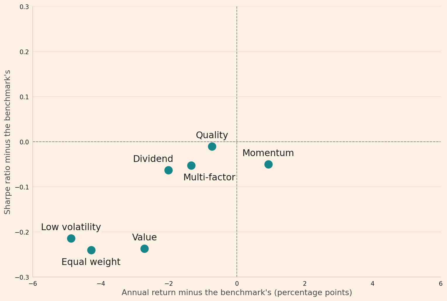
The dashed lines mark a difference of zero. A dot to the right of the vertical line is a strategy whose funds earned more than their benchmarks on average. A dot above the horizontal line is one whose funds had a higher average Sharpe ratio. So, all seven dots are below the horizontal line, and only momentum is to the right of the vertical line.
Limitations
The funds are a selection. I chose large funds that still trade, without checking their sizes against a dated list of assets. Funds that closed are not in the sample, and funds that did well can have grown into the largest. So the 21 funds can show better results than all the smart beta funds that traded in 2015.
Some benchmarks are only similar. For 9 of the 21 funds, the benchmark is the most similar of the five indexes, because the fund’s own index selects from another list of companies. Against an index of exactly that list, these funds’ differences can be larger or smaller. With SPY as every fund’s benchmark, the strategy averages have the same signs.
MSCI USA has no fund fees. The other four benchmarks are ETFs whose returns are after their fees. A fund that tracks MSCI USA earns less than the index, so the funds compared with MSCI USA would have higher differences against such a fund.
One period and no significance test. The averages cover 131 months, and I do not test whether the differences are statistically different from zero. So a small difference, such as quality’s −0.01 in Sharpe ratio, can come from chance.
Conclusion
Did the smart beta rules improve on cap weighting? From November 2015 to September 2026, not on average. In all seven strategies, the funds had a lower average Sharpe ratio than their benchmarks, and only the momentum funds earned more return, with more volatility. Of the 21 funds, 17 had a lower Sharpe ratio than their benchmark.
The takeaway is that, over these 131 months, the cap-weighted benchmarks gave more return per unit of risk than the smart beta funds did on average, in each of the seven strategies.
Appendix: the data
The code below runs first. It downloads the data, chooses one LSEG code per ETF and builds the monthly returns that the steps above compare.
Settings
The funds, their strategies and their benchmarks, and the 131 months. In BENCHMARK, the first 12 funds have the index from which their own index selects, and the last 9 the most similar of the five.
from pathlib import Path

import matplotlib.pyplot as plt
import numpy as np
import pandas as pd

FOLDER = Path.cwd()                          # files are read and written beside this notebook
RETURNS_FILE = FOLDER / "sample_monthly_returns.csv"
INDEX_FILE = FOLDER / "msci_usa_levels.csv"
TBILL_FILE = FOLDER / "tbill_3m.csv"

# From November 2015, the first full month after the youngest fund, SPMO, started trading, to
# September 2026, the last complete month. period_range lists the months from START to END
START, END = "2015-11-01", "2026-09-30"
MONTHS = pd.period_range(START, END, freq="M")
MSCI_USA_RIC = ".dMIUS00000GUS"     # LSEG's code of MSCI USA with gross dividends reinvested

# The 21 funds and their strategies
STRATEGY = {"MTUM": "Momentum", "SPMO": "Momentum", "PDP": "Momentum",
            "QUAL": "Quality", "SPHQ": "Quality", "DGRW": "Quality",
            "VLUE": "Value", "RPV": "Value", "PWV": "Value",
            "USMV": "Low volatility", "SPLV": "Low volatility", "LGLV": "Low volatility",
            "VIG": "Dividend", "SCHD": "Dividend", "VYM": "Dividend",
            "RSP": "Equal weight", "EUSA": "Equal weight", "QQQE": "Equal weight",
            "GSLC": "Multi-factor", "LRGF": "Multi-factor", "QUS": "Multi-factor"}
# Each fund's benchmark
BENCHMARK = {
    # 12 funds: the index from which the fund's own index selects its companies
    "MTUM": "MSCI USA", "QUAL": "MSCI USA", "VLUE": "MSCI USA", "USMV": "MSCI USA",
    "EUSA": "MSCI USA", "QUS": "MSCI USA", "SPMO": "S&P 500", "SPHQ": "S&P 500",
    "RPV": "S&P 500", "SPLV": "S&P 500", "RSP": "S&P 500", "QQQE": "Nasdaq-100",
    # 9 funds whose own index selects from another list of companies: the most similar of the five
    "LRGF": "MSCI USA", "PWV": "S&P 500", "GSLC": "S&P 500", "PDP": "Russell 1000",
    "LGLV": "Russell 1000", "VYM": "Russell 1000", "VIG": "US market", "SCHD": "US market",
    "DGRW": "US market"}
# The series used for each benchmark: an ETF that tracks it, or the MSCI USA index itself
BENCHMARK_SERIES = {"S&P 500": "SPY", "MSCI USA": "MSCI USA", "Russell 1000": "IWB",
                    "US market": "VTI", "Nasdaq-100": "QQQ"}

# The ETFs to download, and each in four forms of LSEG code: the ticker alone and with .K, .Z or
# .O, so the list holds 'MTUM', 'MTUM.K', 'MTUM.Z', 'MTUM.O', 'SPMO', ...
ETFS = [*STRATEGY, "SPY", "IWB", "VTI", "QQQ"]
CANDIDATE_RICS = [ticker + suffix for ticker in ETFS for suffix in ["", ".K", ".Z", ".O"]]
Downloads
One request to LSEG asks for the monthly total returns of the 21 funds and the four benchmark ETFs, and a second for the daily levels of MSCI USA. LSEG can give one ETF several codes, so the first request asks for each ETF with four forms of code: the ticker alone and with .K, .Z or .O.
The Treasury bill rates come from FRED as one file. Each file is saved beside the notebook, so a later run downloads nothing.
# Download the returns again when ETFS has an ETF that the saved file does not have;
# set(a) <= set(b) asks whether every element of a is in b
saved = set()
if RETURNS_FILE.exists():
    saved = set(pd.read_csv(RETURNS_FILE)["Instrument"].str.split(".").str[0])
download_returns = not set(ETFS) <= saved
if download_returns or not INDEX_FILE.exists():
    import lseg.data as ld                   # needs LSEG Workspace running and logged in
    ld.open_session()
    if download_returns:
        # TR.TotalReturn with Frq "M" gives each month's total return in %
        ld.get_data(universe=CANDIDATE_RICS, fields=["TR.TotalReturn.date", "TR.TotalReturn"],
                    parameters={"SDate": START, "EDate": END, "Frq": "M"}
                    ).to_csv(RETURNS_FILE, index=False)
    if not INDEX_FILE.exists():              # from October 2015, for November's return
        ld.get_data(universe=[MSCI_USA_RIC], fields=["TR.PriceClose.date", "TR.PriceClose"],
                    parameters={"SDate": "2015-10-01", "EDate": END, "Frq": "D"}
                    ).to_csv(INDEX_FILE, index=False)
    ld.close_session()
if not TBILL_FILE.exists():
    pd.read_csv("https://fred.stlouisfed.org/graph/fredgraph.csv?id=DTB3"
                ).to_csv(TBILL_FILE, index=False)
One LSEG code per ETF
For each ETF, I keep the code that does not end in .Z and has a return in every month. The code stops if an ETF has no such code or more than one.
The output summarises, across the ETFs, the missing months and the differences in growth between the .Z codes and the codes used. Of the 25 .Z codes, 3 miss a month, while every ETF has a complete code without .Z, so one rule gives every ETF a complete code. Of the 22 complete .Z codes, 3 grew more than 1% less over the 131 months than the code used for the same ETF, and none grew more than 1% more.
returns = pd.read_csv(RETURNS_FILE)
returns.columns = ["ric", "date", "total_return"]         # total_return is in %
returns = returns.dropna()                     # a code without data has empty rows
returns["month"] = pd.to_datetime(returns["date"]).dt.to_period("M")
returns = returns.loc[returns["month"].isin(MONTHS)]
# One return per code and month, the one dated last in the month
returns = returns.sort_values("date").drop_duplicates(["ric", "month"], keep="last")
returns["etf"] = returns["ric"].str.split(".").str[0]      # 'MTUM.K' -> 'MTUM'

# One row per code: its ETF, its number of months and its growth of 1 over those months.
# log1p(x) is log(1 + x), so adding up the logs and taking exp() compounds the returns
returns["log_growth"] = np.log1p(returns["total_return"] / 100)
codes = returns.groupby(["etf", "ric"]).agg(months=("month", "size"),
                                            log_growth=("log_growth", "sum")).reset_index()
codes["growth"] = np.exp(codes["log_growth"])
codes["complete"] = codes["months"] == len(MONTHS)
codes["ends_in_z"] = codes["ric"].str.endswith(".Z")

# For each ETF, the complete code that does not end in .Z; ~ turns True into False and False
# into True. assert stops the run with its message when the condition is False: is_unique asks
# whether no ETF appears twice, and subtracting one set from another keeps the ETFs without
# such a code. An f-string puts the value in braces into the text
chosen = codes.loc[codes["complete"] & ~codes["ends_in_z"]]
assert chosen["etf"].is_unique, "an ETF has two such codes"
missing = set(ETFS) - set(chosen["etf"])
assert not missing, f"no such code for {missing}"
chosen_rics = chosen["ric"]
print(f"ETFs with one such code: {len(chosen)} of {len(ETFS)}")

# Why the .Z codes are left out, counted across the ETFs: the .Z codes with a missing month,
# and each complete .Z code's growth against the growth of the code used for the same ETF.
# suffixes names the two growth columns growth_z and growth_used
z_codes = codes.loc[codes["ends_in_z"]]
print(f".Z codes with a missing month: {(~z_codes['complete']).sum()} of {len(z_codes)}")
compared = z_codes.loc[z_codes["complete"]].merge(chosen[["etf", "growth"]], on="etf",
                                                  suffixes=("_z", "_used"))
growth_ratio = compared["growth_z"] / compared["growth_used"]
print(f"Complete .Z codes that grew more than 1% less than the code used: "
      f"{(growth_ratio < 0.99).sum()} of {len(compared)}")
print(f"Complete .Z codes that grew more than 1% more than the code used: "
      f"{(growth_ratio > 1.01).sum()} of {len(compared)}")
ETFs with one such code: 25 of 25
.Z codes with a missing month: 3 of 25
Complete .Z codes that grew more than 1% less than the code used: 3 of 22
Complete .Z codes that grew more than 1% more than the code used: 0 of 22Monthly returns
The chosen codes give one column of monthly returns per ETF. MSCI USA’s monthly return is the change in its level from one month end to the next. The cash return of each month comes from the Treasury bill rate at the end of the month before, a rate known before the month starts.
# One row per month and one column per ETF, with the returns as decimals
monthly = returns.loc[returns["ric"].isin(chosen_rics)].pivot(index="month", columns="etf",
                                                              values="total_return") / 100

# MSCI USA's monthly return is the change in its level from one month end to the next.
# resample("ME") groups the days by calendar month, last() takes each month's last level, and
# to_period("M") turns the month-end dates into months; assigning to monthly matches the rows
msci_levels = pd.read_csv(INDEX_FILE, parse_dates=["Date"])
msci_levels = msci_levels.loc[msci_levels["Instrument"] == MSCI_USA_RIC]
msci_levels = msci_levels.set_index("Date")["Price Close"]
monthly["MSCI USA"] = msci_levels.resample("ME").last().pct_change().to_period("M")
# notna() marks each value that is present, and .all().all() asks whether every value is
assert monthly.notna().all().all(), "a monthly return is missing"

# The cash return of a month: one twelfth of the 3-month T-bill rate, an annual rate in %, at
# the end of the month before. FRED leaves bond-market holidays empty, and last() skips them;
# shift(1) moves each month-end rate to the next month
tbill = pd.read_csv(TBILL_FILE, na_values=".", parse_dates=["observation_date"],
                    index_col="observation_date")["DTB3"]
month_end_rate = tbill.resample("ME").last().shift(1).to_period("M")
cash = month_end_rate.loc[monthly.index] / 100 / 12
# sub(cash, axis=0) subtracts each month's cash return from every column of that month
excess = monthly.sub(cash, axis=0)
# shape[1] is the number of columns
print(f"{len(monthly)} months, {monthly.index[0].strftime('%b %Y')} to "
      f"{monthly.index[-1].strftime('%b %Y')}, for {monthly.shape[1]} series")
131 months, Nov 2015 to Sep 2026, for 26 seriesThe 26 series are the 21 funds, the four benchmark ETFs and MSCI USA, each with a return in all 131 months.
Read next
- How to do factor investing How a factor portfolio is selected, weighted and rebalanced, with its trading costs.
- Does your backtested Sharpe ratio show a real edge? How uncertain a Sharpe ratio estimated from a few years of returns is.
- Does announcing trades still hurt index investors? The stocks entering and leaving the index behind USMV, one of the low-volatility funds here.
Disclaimer: an empirical study for discussion purposes, not investment advice. The design is descriptive and not causal. Past performance does not guarantee future returns.
Sources: monthly total returns of the ETFs and daily levels of the MSCI USA index with gross dividends reinvested from LSEG Workspace (licensed); I do not reproduce the raw data here. The 3-month Treasury bill rate (DTB3) from FRED, Federal Reserve Bank of St. Louis. SPMO’s start in October 2015 from Invesco’s fund information.