Do income ETFs pay off?
Of 96 US income ETFs with at least three years of returns, seven paid out 10% or more of their price a year, 12% on average. Their total return was 10% a year. SPY, the S&P 500 ETF, returned 16% a year over the same months.
An income ETF is an ETF that pays its investors cash regularly, often monthly, from the dividends of its stocks or from selling call options on them. Each payment is called a distribution. A distribution creates no value. The cash moves from the fund to the investor, so the fund is worth less. For example, if nothing else changes, a share priced at $100 is worth $99 after a distribution of $1. Its investor holds $99 in the fund and $1 in cash, the same $100 as before.
Only what a fund earns adds to its total return
An investor’s total return includes the distributions and the change in the price,
\[\text{total return} = \frac{\text{price at the end} + \text{distributions}}{\text{price at the start}} - 1.\]
For example, a share bought at $100 that distributes $1 and ends at $99 has a total return of (99 + 1) / 100 − 1 = 0%. The $1 the investor receives is the $1 the price loses. So the total return is larger only when the fund earns more, from dividends, option premiums or capital gains.
The money for a distribution comes from the fund’s dividends, option premiums and realized capital gains. When these add up to less than the distribution, the fund pays the rest by selling some of its stocks. That part is a return of capital, and the fund holds fewer stocks. The chart follows one share of a hypothetical fund for a year. In that year, the fund has no costs, its stocks’ prices do not change, and the call options it sells expire worthless.
When a fund pays out more than its total return, its price falls by the difference. On average, the seven funds paying 10% or more paid out 12% a year, more than their total return of 10%, and their price fell 2% a year.
A covered call gives up gains above the strike price
A covered call means holding stocks and selling call options on them, a strategy many income ETFs use. A call option on the S&P 500 pays its buyer the amount by which the index ends above the strike price on the expiry date, and the buyer pays the seller a premium for it at the start.
Take a fund that holds the S&P 500 and each month sells a one-month at-the-money call on it. Say the index is at 5,000 and the premium is 100, which is 2% of 5,000. If the index rises 5% to 5,250, the fund’s stocks gain 250, and the fund pays the buyer 5,250 − 5,000 = 250. It also keeps the premium, so in total it gains 250 − 250 + 100 = 100, or 2%. If the index falls 5% to 4,750, the option pays nothing, because the index ended below the strike price. The fund’s stocks lose 250, and it keeps the premium, so in total it loses 250 − 100 = 150, or 3%. So the fund’s return for the month is
\[\text{fund's return} = \text{premium} + \min(\text{index's return},\ 0),\]
where the premium and the index’s return are percentages of the index’s level at the start of the month. The formula uses the index’s price return and leaves out dividends and costs.
The chart shows this payoff for monthly index returns from −10% to 10%.
The fund returns more than the index in a month when the index falls or rises by less than the premium. It returns less in a month when the index rises by more than the premium.
92 of 96 income ETFs returned less than SPY
Of the 96 income ETFs, 92 had a lower annual return than SPY over the same months, and 91 had a lower Sharpe ratio. I call a fund an option-income fund when its name says it earns income from options, with words such as covered call or buy-write. I take every US-based ETF in the US equity income class of Lipper, LSEG’s fund classification, and the option-income funds on broad US stocks from other classes. Of these 166 funds, 96 have at least 36 months of returns, from 2003 for the oldest to September 2026, and 19 of the 96 are option-income funds. I compare each fund with SPY over the fund’s own months.
Annual returns are compounded. A fund’s payout is its annualized distribution yield, averaged over its months. I put the funds into three groups by their payout: under 5% a year, 5% to 10%, and 10% or more.
The Sharpe ratio is
\[\text{Sharpe ratio} = \frac{\text{average excess return}}{\text{its standard deviation}} \times \sqrt{12},\]
where the excess return is a fund’s monthly total return minus a twelfth of the 3-month Treasury bill rate, and √12 annualizes the monthly ratio.
The chart puts SPY at the centre and moves each payout group to its funds’ average differences from SPY. Across is the difference in annual return, and up is the difference in Sharpe ratio.
Of the 30 funds paying 5% or more, 18 are option-income funds, and their two groups trailed SPY by 6.8 and 6.0 percentage points a year on average. Of the 66 funds paying under 5%, 1 is an option-income fund, and their group trailed SPY by 4.4. Every group’s Sharpe ratio was lower than SPY’s, so the funds also earned less per unit of risk.
Limitations
The groups mix years and strategies. Each fund is compared with SPY over its own months, but the funds in a group started in different years, and each fund counts once, however many months it has. So the averages describe these 96 funds and do not show what a higher payout causes.
Some funds and distributions may be missing. The 36-month requirement leaves out 70 funds, 18 of which had closed, and LSEG’s search may also miss closed funds, so the results can have survivorship bias. Across 17 funds, 46 calendar years had fewer payment dates than the fund’s usual number. Such a year can lack a distribution in the data or reflect a change in payment frequency. Giving each of these years the fund’s usual number of payments, at its median distribution, changes a group’s average difference from SPY’s annual return by at most 0.06 percentage points.
The returns are before taxes. How a distribution is taxed depends on the investor, the account and how much of it the fund reports as a return of capital. That tax label can differ from the return of capital in the first chart.
Conclusion
The takeaway is that a distribution moves money from a fund’s price into the investor’s cash, so the measure for comparing an income ETF with other funds is its total return. An investor with $100 in a fund who needs $1 in cash can also sell $1 of shares and keep $99 in the fund, as with a distribution of $1.
Appendix: the code
The notebook reads the prices and distributions from LSEG Workspace and the 3-month Treasury bill rate from FRED, and saves each download, so that a later run reads the saved files. I show the code without running it here, with the output of my run. Because the LSEG data is licensed, the code prints only counts and averages.
from pathlib import Path
import json

import matplotlib.pyplot as plt
import numpy as np
import pandas as pd

# Path.cwd() is the folder this notebook runs in, and / joins a folder and a file name
FOLDER = Path.cwd()
UNIVERSE_FILE = FOLDER / "nr79_universe.csv"               # the candidate funds, LSEG search
PRICES_FILE = FOLDER / "nr79_monthly_prices.csv"           # month-end closing prices, LSEG
DISTRIBUTIONS_FILE = FOLDER / "nr79_distributions.csv"     # each distribution, LSEG
TBILL_FILE = FOLDER / "tbill_3m.csv"                       # the 3-month T-bill rate, FRED
NUMBERS_FILE = FOLDER / "income_etfs_numbers.json"         # the numbers the post's charts draw
CHART_FILE = FOLDER / "income_etfs.png"                    # the chart that previews the post

# From January 2003, before the oldest income ETFs started trading, to September 2026, the last
# complete month. period_range lists the months from START to END
START, END = "2003-01-01", "2026-09-30"
MONTHS = pd.period_range(START, END, freq="M")
MIN_MONTHS = 36                                      # the fewest months of returns a fund needs
BENCHMARK = "SPY"                                    # LSEG's code of the S&P 500 ETF
CHUNK = 25                                           # codes per LSEG request

# The words in a fund's name that mark option income, and the words that mark option income on
# something other than broad US stocks. In a regular expression, | means or, (?:...) groups words
# without keeping the match, and \b marks the edge of a word, so that 'gold' matches 'Gold
# Miners' but not 'Goldman'. YieldMax names its single-stock funds '... Option Income Strategy'
OPTION_WORDS = r"covered call|buywrite|buy-write|premium income|option income|options income"
OPTION_WORDS += r"|high income|enhanced income|covered-call|buy write"
NOT_BROAD_US = r"\b(?:bitcoin|ether|ethereum|solana|xrp|crypto|gold|silver|oil|miners|eafe"
NOT_BROAD_US += r"|emerging|kweb|mstr|bmnr|short|option income strategy|real estate|reit"
NOT_BROAD_US += r"|semiconductor|cybersecurity|ai|magnificent|fang|fund of|buffer|barrier)\b"

# The payout groups: the edges of each band of payout a year, in percent, and a name for each
# band. np.inf is infinity, so the last band has no upper edge
EDGES = [0, 5, 10, np.inf]
GROUPS = ["under 5%", "5% to 10%", "10% or more"]def open_lseg():
"""Open the LSEG session with nr73b's patch: open_lseg() returns the lseg.data module, ready
to use. Needs LSEG Workspace running and logged in."""
import httpx
import lseg.data as ld
ld.get_config().set_param("http.request-timeout", 300)
try:
ld.open_session()
except AttributeError: # lseg-data 2.1.1 with httpx 0.28: no proxy
for client in (httpx.Client, httpx.AsyncClient):
original = client.__init__
def patched(self, *args, _original=original, **kwargs):
if isinstance(kwargs.get("proxy"), dict):
kwargs["proxy"] = next((value for value in kwargs["proxy"].values() if value),
None)
return _original(self, *args, **kwargs)
client.__init__ = patched
ld.open_session()
return ld
if not UNIVERSE_FILE.exists():
ld = open_lseg()
# US-domiciled ETFs, primary listings, in a US equity class or an Alternative class
search_filter = ("IssuerDomicileCountryName eq 'United States'"
" and AssetCategoryName eq 'Fund Unit/Exchange Traded Fund'"
" and IsPrimaryRIC eq true"
" and (startswith(IssueLipperGlobalSchemeName, 'Equity US')"
" or startswith(IssueLipperGlobalSchemeName, 'Alternative'))")
found = ld.discovery.search(view=ld.discovery.Views.FUND_QUOTES, filter=search_filter,
select="RIC,DTSubjectName,IssueLipperGlobalSchemeName", top=5000)
ld.close_session()
# top=5000 is the most rows one search returns, so fewer rows mean the list is complete
assert len(found) < 5000, "the search stopped at its limit of 5,000 rows"
found.to_csv(UNIVERSE_FILE, index=False)
universe = pd.read_csv(UNIVERSE_FILE)
universe.columns = ["ric", "name", "lipper_class"]
is_income = universe["lipper_class"] == "Equity US Income"
# str.contains(..., case=False) asks whether a name contains a pattern, ignoring capitals
names_options = universe["name"].str.contains(OPTION_WORDS, case=False)
not_broad = universe["name"].str.contains(NOT_BROAD_US, case=False)
# Every fund the search found is in a US equity or an Alternative class. | is or, & is and, and
# ~ turns True into False and False into True
option_income = ~is_income & names_options & ~not_broad
candidates = universe.loc[is_income | option_income]
print(f"Funds found: {len(universe)}; Equity US Income: {is_income.sum()}; other funds named "
f"for option income: {(~is_income & names_options).sum()}, of them on broad US stocks: "
f"{option_income.sum()}")
assert candidates["ric"].is_unique, "a fund appears twice"Funds found: 2907; Equity US Income: 121; other funds named for option income: 152, of them on broad US stocks: 45# The codes to download: the candidates and SPY. tolist() turns a column into a list
rics = candidates["ric"].tolist() + [BENCHMARK]
def download(fields, parameters):
"""One LSEG table for all codes, asked for CHUNK codes at a time: download(["TR.ClosePrice"],
{...}) gives the rows of every code, one after another. rics[first:first + CHUNK] is a
position slice, which stops before its end."""
tables = []
for first in range(0, len(rics), CHUNK):
answer = ld.get_data(universe=rics[first:first + CHUNK], fields=fields,
parameters=parameters)
# LSEG can answer a request with empty rows only, when its service fails. Then the run
# stops before anything is saved, so the next run downloads again
assert answer.dropna().shape[0] > 0, "LSEG gave no data for a request: restart Workspace"
tables.append(answer)
return pd.concat(tables, ignore_index=True)
# LSEG lists every code it was asked for, in an empty row when it has no data for it, so a
# saved file counts when it lists every code; set(a) <= set(b) asks whether every element of a
# is in b. An answer without any data is never saved (see download)
saved_prices = set()
saved_distributions = set()
if PRICES_FILE.exists():
saved_prices = set(pd.read_csv(PRICES_FILE)["Instrument"])
if DISTRIBUTIONS_FILE.exists():
saved_distributions = set(pd.read_csv(DISTRIBUTIONS_FILE)["Instrument"])
download_prices = not set(rics) <= saved_prices
download_distributions = not set(rics) <= saved_distributions
if download_prices or download_distributions:
ld = open_lseg()
if download_prices:
# TR.ClosePrice with Frq "M" gives each month's last closing price
download(["TR.ClosePrice.date", "TR.ClosePrice"],
{"SDate": START, "EDate": END, "Frq": "M"}).to_csv(PRICES_FILE, index=False)
if download_distributions:
download(["TR.DivExDate", "TR.DivAdjustedGross"],
{"SDate": START, "EDate": "2026-12-31"}).to_csv(DISTRIBUTIONS_FILE, index=False)
ld.close_session()
if not TBILL_FILE.exists():
pd.read_csv("https://fred.stlouisfed.org/graph/fredgraph.csv?id=DTB3"
).to_csv(TBILL_FILE, index=False)prices = pd.read_csv(PRICES_FILE)
prices.columns = ["ric", "date", "price"]
prices = prices.dropna() # a code without data has empty rows
# str[:10] keeps the first ten characters of LSEG's date text, the year, month and day, and
# to_period("M") turns each date into its month, such as 2003-01
prices["month"] = pd.to_datetime(prices["date"].str[:10]).dt.to_period("M")
prices = prices.loc[prices["month"].isin(MONTHS)]
# One price per code and month, the one dated last in the month; then one row per month and one
# column per code. reindex puts in every month and every code, a missing one empty
prices = prices.sort_values("date").drop_duplicates(["ric", "month"], keep="last")
month_end_price = prices.pivot(index="month", columns="ric", values="price")
month_end_price = month_end_price.reindex(index=MONTHS, columns=rics)
distributions = pd.read_csv(DISTRIBUTIONS_FILE)
distributions.columns = ["ric", "ex_date", "amount"]
# Rows without an amount are announced distributions that have not been paid yet
distributions = distributions.dropna()
distributions["month"] = pd.to_datetime(distributions["ex_date"].str[:10]).dt.to_period("M")
distributions = distributions.loc[distributions["month"].isin(MONTHS)]
# A distribution paid in two parts on one date has two rows, and both count in the sums below.
# duplicated() marks a row that repeats an earlier one in all three columns, the same code, date
# and amount: one payment listed twice, which is counted once
repeated = distributions.duplicated(["ric", "ex_date", "amount"])
print(f"Distributions listed twice with the same code, date and amount, counted once: "
f"{repeated.sum()}")
distributions = distributions.loc[~repeated]
# pivot_table sums each code's distributions in each month; reindex lines the table up with the
# prices, and fillna(0) says that a month without an ex-dividend date paid nothing
paid = distributions.pivot_table(index="month", columns="ric", values="amount", aggfunc="sum")
paid = paid.reindex(index=month_end_price.index, columns=month_end_price.columns).fillna(0)
# shift(1) takes the price at the end of the month before; a month without both prices has no
# return
price_before = month_end_price.shift(1)
monthly = (month_end_price + paid) / price_before - 1
payout = paid / price_before
price_change = month_end_price / price_before - 1
# A month whose price equals the month before exactly may be a stale price. The code counts such
# months and leaves them as they are
stale = (price_change == 0).sum().sum()
print(f"Codes with prices: {month_end_price.notna().any().sum()} of {len(rics)}; months with a "
f"price equal to the month before: {stale}")
# FRED leaves bond-market holidays empty, and last() skips them; shift(1) moves each month-end
# rate to the next month, and sub(risk_free, axis=0) subtracts each month's risk-free return
# from every column of that month
tbill = pd.read_csv(TBILL_FILE, na_values=".", parse_dates=["observation_date"],
index_col="observation_date")["DTB3"]
month_end_rate = tbill.resample("ME").last().shift(1).to_period("M")
risk_free = month_end_rate.reindex(MONTHS) / 100 / 12
excess = monthly.sub(risk_free, axis=0)Distributions listed twice with the same code, date and amount, counted once: 1
Codes with prices: 167 of 167; months with a price equal to the month before: 19rows = []
too_short = 0
too_short_closed = 0
with_gap = 0
for ric in candidates["ric"]:
has_price = month_end_price[ric].notna()
if not has_price.any():
too_short += 1 # += adds to the count: no prices at all
continue
# The fund's months: from the month after its first price, its first full month, to its last
# price. idxmax() gives the first True, the first month with a price, and a month plus 1 is
# the next; has_price.loc[has_price] keeps the months with a price, and max() the last
first_full = has_price.idxmax() + 1
last = has_price.loc[has_price].index.max()
# A distribution larger than half the price pays out a closing fund's value: the fund's months
# end the month before the first such distribution. A month minus 1 is the month before
liquidations = payout.loc[payout[ric] > 0.5].index
ended_early = len(liquidations) > 0
if ended_early:
last = liquidations.min() - 1
months = pd.period_range(first_full, last, freq="M")
if len(months) < MIN_MONTHS:
too_short += 1
# LSEG marks a closed fund's code with ^ and the month and year it closed
if "^" in ric:
too_short_closed += 1
continue
# DataFrame.loc[rows, columns] selects rows and columns: the months and the two codes
pair = monthly.loc[months, [ric, BENCHMARK]]
# notna() marks each value that is present, and .all().all() asks whether every value is
if not pair.notna().all().all():
with_gap += 1
continue
# A split the prices are not adjusted for would show as a monthly return of 50% or more;
# abs() drops the sign
assert pair[ric].abs().max() < 0.5, f"{ric}: a monthly return of 50% or more, a split?"
pair_excess = excess.loc[months, [ric, BENCHMARK]]
assert pair_excess.notna().all().all(), f"{ric}: a month without a T-bill rate"
# ** raises to a power, and prod() multiplies the monthly growth factors
annual = ((1 + pair).prod() ** (12 / len(months)) - 1) * 100
sharpe = pair_excess.mean() / pair_excess.std() * np.sqrt(12)
# The annual price change, without distributions: from the end of the month before the fund's
# first full month to the end of its last month
price_a_year = ((month_end_price.loc[months[-1], ric] / month_end_price.loc[months[0] - 1, ric])
** (12 / len(months)) - 1) * 100
rows.append({"ric": ric, "closed": "^" in ric, "ended early": ended_early,
"first month": months[0], "last month": months[-1], "months": len(months),
"annual return": annual[ric], "SPY annual return": annual[BENCHMARK],
"return gap": annual[ric] - annual[BENCHMARK],
"Sharpe gap": sharpe[ric] - sharpe[BENCHMARK],
"payout": payout.loc[months, ric].mean() * 12 * 100,
"price change": price_a_year})
funds = pd.DataFrame(rows).merge(candidates[["ric", "name"]], on="ric", how="left")
print(f"Funds compared: {len(funds)}, of them closed: {funds['closed'].sum()}, ended the month "
f"before a final distribution: {funds['ended early'].sum()}; left out with fewer than "
f"{MIN_MONTHS} months: {too_short}, of them closed: {too_short_closed}; left out with a gap "
f"in their months: {with_gap}")
# Checks on the funds compared: one still trading whose prices stop early, and one that paid
# nothing in all its months, would each point to missing data
stops_early = ~funds["closed"] & (funds["last month"] < MONTHS[-1])
print(f"Funds still trading whose prices stop before {MONTHS[-1]}: {stops_early.sum()}; funds "
f"without any distribution in their months: {(funds['payout'] == 0).sum()}")
# A check for missing distributions: each fund's number of payment dates, with an amount above
# zero, in every calendar year its months cover from January to December, and the years with
# fewer than the fund's usual number, the median. Such a year needs a look: a missing payment, a
# fund that changed how often it pays, or a payment that crossed a year end. LSEG lists some
# distributions with an amount of zero, which are not payments
payment_dates = distributions.loc[distributions["amount"] > 0].drop_duplicates(["ric", "ex_date"])
payments = payment_dates.groupby(["ric", payment_dates["month"].dt.year]).size()
flagged_years = 0
flagged_funds = 0
# A check of what missing payments could change, under its own assumptions: each payment date a
# flagged year lacks, against the fund's usual number rounded up, is added in December of that year
# at the fund's median distribution. paid * 0 is a table of zeros with the months and codes of paid
added = paid * 0
for index, row in funds.iterrows():
# The years from January to December inside the fund's months; pd.Period(..., "M") is a month
years = []
for year in range(row["first month"].year, row["last month"].year + 1):
covered = (row["first month"] <= pd.Period(f"{year}-01", "M")
and row["last month"] >= pd.Period(f"{year}-12", "M"))
if covered:
years.append(year)
if len(years) < 2:
continue
# payments.loc[ric] is the fund's count per year; reindex puts 0 in a year without a payment
per_year = payments.loc[row["ric"]].reindex(years, fill_value=0)
fewer = (per_year < per_year.median()).sum()
if fewer > 0:
flagged_years += fewer
flagged_funds += 1
usual = per_year.median()
median_distribution = distributions.loc[(distributions["ric"] == row["ric"])
& (distributions["amount"] > 0), "amount"].median()
# items() gives each year and its count, and np.ceil rounds up
for year, count in per_year.loc[per_year < usual].items():
added.loc[pd.Period(f"{year}-12", "M"), row["ric"]] += np.ceil(usual - count) * median_distribution
print(f"Whole years with fewer payment dates than the fund's usual number: {flagged_years}, in "
f"{flagged_funds} of {len(funds)} funds")
# Each fund's return gap again, with the payments added and the payout groups as they are. The
# check does not show the largest possible effect: a payment missing from the data can have
# another amount or date, and a year can have fewer payment dates without a missing payment, when
# a fund changes how often it pays
monthly_added = (month_end_price + paid + added) / price_before - 1
gaps_added = []
for index, row in funds.iterrows():
months = pd.period_range(row["first month"], row["last month"], freq="M")
pair = monthly_added.loc[months, [row["ric"], BENCHMARK]]
annual = ((1 + pair).prod() ** (12 / len(months)) - 1) * 100
gaps_added.append(annual[row["ric"]] - annual[BENCHMARK])
funds["return gap, payments added"] = gaps_added
# A second check of the distributions, against totals the funds publish, in dollars a share:
# SPY's per year, State Street's published amounts added up, and TPHD's in 2021, as its annual
# report gives it, rounded to the cent. The sums use distributions, the same rows as the returns,
# so that two parts paid on one date both count. A total agrees when it is within half a cent of
# the published one
PUBLISHED = {("SPY", 2022): 6.32068, ("SPY", 2023): 6.633813, ("SPY", 2024): 7.06504,
("TPHD.K", 2021): 0.60}
agree = 0
for (ric, year), published in PUBLISHED.items():
chosen_rows = distributions.loc[(distributions["ric"] == ric)
& (distributions["month"].dt.year == year)]
if abs(chosen_rows["amount"].sum() - published) < 0.005:
agree += 1
print(f"Yearly totals of distributions a share within half a cent of the published total: "
f"{agree} of {len(PUBLISHED)}")
# The payout groups: pd.cut puts each payout into the band between two edges, with right=False
# so that a payout of exactly 5% falls in "5% to 10%"
funds["group"] = pd.cut(funds["payout"], EDGES, labels=GROUPS, right=False)
# True or False for each fund, so that sum() counts the funds in a group. A fund counts as option
# income when its name has one of the option words, in any Lipper class
funds["option income"] = funds["name"].str.contains(OPTION_WORDS, case=False)
funds["return ahead"] = funds["return gap"] > 0
funds["Sharpe ahead"] = funds["Sharpe gap"] > 0
# One row per group; observed=True keeps only the groups that have funds, and agg gives each new
# column as (column, how): size counts the rows, mean averages and sum counts the True values
groups = funds.groupby("group", observed=True).agg(
funds=("ric", "size"), closed=("closed", "sum"), option_income=("option income", "sum"),
payout=("payout", "mean"), price_change=("price change", "mean"),
annual_return=("annual return", "mean"),
spy_return=("SPY annual return", "mean"),
return_gap=("return gap", "mean"), sharpe_gap=("Sharpe gap", "mean"),
return_ahead=("return ahead", "sum"), sharpe_ahead=("Sharpe ahead", "sum"))
print("\nAverages of each payout group (payout, price change, returns and return gap in % a year; spy_return")
print("is SPY's annual return over the same months as each fund):")
print(groups.round(2).to_string())
print(f"\nAll {len(funds)} funds: return ahead of SPY {funds['return ahead'].sum()}, Sharpe "
f"ratio ahead of SPY {funds['Sharpe ahead'].sum()}")
# The check: how much the payments added change each group's average return gap
change = funds.groupby("group", observed=True)["return gap, payments added"].mean() - groups["return_gap"]
print(f"With the usual number of payments in every flagged year, a group's average return gap "
f"changes by at most {change.abs().max():.2f} percentage points")Funds compared: 96, of them closed: 5, ended the month before a final distribution: 0; left out with fewer than 36 months: 70, of them closed: 18; left out with a gap in their months: 0
Funds still trading whose prices stop before 2026-09: 0; funds without any distribution in their months: 0
Whole years with fewer payment dates than the fund's usual number: 46, in 17 of 96 funds
Yearly totals of distributions a share within half a cent of the published total: 4 of 4
Averages of each payout group (payout, price change, returns and return gap in % a year; spy_return
is SPY's annual return over the same months as each fund):
funds closed option_income payout price_change annual_return spy_return return_gap sharpe_gap return_ahead sharpe_ahead
group
under 5% 66 4 1 2.71 7.87 10.85 15.28 -4.44 -0.28 2 2
5% to 10% 23 0 12 7.61 1.56 9.61 16.39 -6.78 -0.37 1 1
10% or more 7 1 6 11.73 -2.37 9.85 15.86 -6.01 -0.28 1 2
All 96 funds: return ahead of SPY 4, Sharpe ratio ahead of SPY 5
With the usual number of payments in every flagged year, a group's average return gap changes by at most 0.06 percentage points# The post's charts draw these numbers, saved at full precision. int() turns numpy's whole
# numbers into the type JSON stores, and str() writes a month as text, such as 2026-09
group_numbers = {}
for group, row in groups.iterrows():
group_numbers[group] = {"funds": int(row["funds"]), "option_income": int(row["option_income"]),
"payout": row["payout"], "price_change": row["price_change"],
"annual_return": row["annual_return"],
"spy_return": row["spy_return"], "return_gap": row["return_gap"],
"sharpe_gap": row["sharpe_gap"],
"return_ahead": int(row["return_ahead"]),
"sharpe_ahead": int(row["sharpe_ahead"])}
numbers = {"groups": group_numbers, "order": GROUPS, "funds": len(funds),
"option_income": int(funds["option income"].sum()), "closed": int(funds["closed"].sum()),
"return_ahead": int(funds["return ahead"].sum()),
"sharpe_ahead": int(funds["Sharpe ahead"].sum()),
"flagged_years": int(flagged_years), "flagged_funds": flagged_funds,
"added_payments_change": float(change.abs().max()),
"candidates": len(candidates), "left_out_short": too_short,
"left_out_short_closed": too_short_closed, "left_out_gap": with_gap,
"first_year": int(funds["first month"].min().year), "last_month": str(MONTHS[-1])}
# json.dumps writes the dictionary as text, and indent=1 puts each entry on its own line
NUMBERS_FILE.write_text(json.dumps(numbers, indent=1), encoding="utf-8")
print(f"Saved {NUMBERS_FILE.name}")Saved income_etfs_numbers.json# The site's chart colours: the cream background, the text, the light grid lines, the pale frame
# and the axis labels
BG, INK, GRID, SPINE, AXIS_TEXT = "#FCEFE3", "#1f1f1f", "#EADCCC", "#D5C6B4", "#4a4a4a"
TEAL = "#17868A"
# The figure and its chart, 12 by 8 inches; dashed lines (ls="--") of width 1 (lw) at zero
figure, axis = plt.subplots(figsize=(12, 8))
axis.axhline(0, color="#888888", lw=1, ls="--")
axis.axvline(0, color="#888888", lw=1, ls="--")
# SPY is at zero on both axes, where the dashed lines cross
axis.annotate("SPY", (0, 0), xytext=(10, 10), textcoords="offset points", fontsize=14,
color=AXIS_TEXT)
# s is each dot's area, and zorder=3 draws the dots above the lines
axis.scatter(groups["return_gap"], groups["sharpe_gap"], s=160, color=TEAL, zorder=3)
# annotate writes each group's payout band and number of funds in three lines 14 points from its
# dot, where a point is 1/72 inch: right of the first group's dot, left of the second's and above
# the third's, where the other dots leave room. \n starts a new line, ha and va set which side of
# the text is at that place, and iterrows() gives each row of groups with its label
PLACES = {"under 5%": ((14, 0), "left", "center"), "5% to 10%": ((-14, 0), "right", "center"),
"10% or more": ((0, 14), "center", "bottom")}
for group, row in groups.iterrows():
offset, ha, va = PLACES[group]
axis.annotate(f"payout\n{group}\n{row['funds']:.0f} funds", (row["return_gap"], row["sharpe_gap"]),
xytext=offset, textcoords="offset points", ha=ha, va=va, fontsize=14, color=INK)
axis.set_xlabel("Annual return minus SPY's (percentage points)", fontsize=13, color=AXIS_TEXT)
axis.set_ylabel("Sharpe ratio minus SPY's", fontsize=13, color=AXIS_TEXT)
# Axis limits symmetric around zero, a little wider than the farthest dot; np.ceil rounds up
x_limit = np.ceil(groups["return_gap"].abs().max()) + 3
y_limit = np.ceil(groups["sharpe_gap"].abs().max() * 10) / 10 + 0.1
axis.set_xlim(-x_limit, x_limit)
axis.set_ylim(-y_limit, y_limit)
# The site's chart style: a light grid on the y-axis only, drawn behind the dots, no top and right
# borders, and tick labels without tick marks (length=0)
figure.patch.set_facecolor(BG)
axis.set_facecolor(BG)
axis.grid(True, axis="y", color=GRID)
axis.set_axisbelow(True)
axis.spines[["top", "right"]].set_visible(False)
axis.spines[["left", "bottom"]].set_color(SPINE)
axis.tick_params(axis="both", length=0, colors=INK, pad=6)
# 150 dots per inch, cropped to the chart, with the background colour; show() draws it below
plt.savefig(CHART_FILE, dpi=150, bbox_inches="tight", facecolor=BG)
plt.show()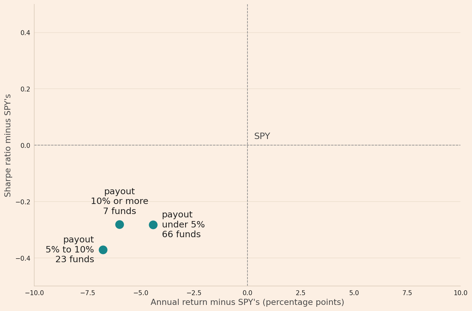
Read next
- Do the highest-yielding stocks beat the S&P 500? The 30 highest-yielding US stocks returned 7.9% a year after trading costs from 2012 to 2026, against 15.0% for the S&P 500.
- How smart are smart beta ETFs? From November 2015 to September 2026, the funds of all seven smart beta strategies had a lower average Sharpe ratio than their cap-weighted benchmarks.
- How do ETFs work? Creation and redemption, step by step Why an ETF’s price stays close to its net asset value, and how its shares are created and redeemed.
Disclaimer: an empirical study for discussion purposes, not investment advice. The design is descriptive and not causal. Past performance does not guarantee future returns.
Data: month-end closing prices and distributions of the ETFs from LSEG Workspace (licensed), and the 3-month Treasury bill rate (Federal Reserve Board) through FRED. I do not reproduce the raw files here.