How to do factor investing

How to turn value and momentum into one score, select and weight 100 stocks, and rebalance them with trading costs, on simulated data.

Factor investing selects and weights stocks by fixed rules based on their characteristics, such as value, how cheap a stock is relative to its fundamentals, and momentum, its return over the past year. Combining several characteristics is multifactor investing. The previous post examined whether a characteristic predicts returns; this post uses value and momentum to build and maintain a portfolio, with one example on simulated data.

Here the two characteristics rank stocks for a long-only portfolio, which owns stocks and never sells borrowed shares. An academic factor return such as HML, the value factor of Fama and French (1993), is the return of a long-short portfolio, which buys stocks with high book-to-market ratios and sells borrowed shares of stocks with low ones.

Simulating the data

The simulated data is a daily panel of stock data: one row per stock and trading day, with the date, the ticker, the total return, the market cap, the book equity and the sector of 500 stocks from January 2004 to December 2025. Historical fundamentals must be the values known at the time, so each day’s book equity is the latest published value, repeated until the next report. The portfolio runs over the last 240 months, 2006 to 2025. In short, with every rule in the box below:

• Returns. Each month, a stock’s total return is its expected return plus a market, a sector and a stock-specific shock, larger for smaller firms, and the stock’s daily returns compound to it. Market cap grows with the total return less dividends.
• Fundamentals. Book equity, assets minus liabilities, grows by earnings less dividends, and each annual report is published 2 to 4 months after the fiscal year-end.
• The assumed premium. The expected return is 0.8% a month in the middle of both rankings, and 0.3 percentage points a month higher at the top of the value ranking than at the bottom; the same holds for momentum.

These are assumptions, so any outperformance below illustrates them and cannot show that the strategy works in real markets.

NoteHow the data is simulated

The simulation first runs month by month, so one observation is a stock-month. At the start, I draw for each stock its sector, one of ten, each equally likely; its market beta \(\beta_i\), which multiplies the market shock in its return, equally likely anywhere between 0.7 and 1.3; its market cap, whose logarithm is drawn from a normal distribution, the bell-shaped distribution, centred on the logarithm of $10 billion with a standard deviation, the typical distance from the centre, of 1; its payout ratio, the share of earnings paid as dividends, equally likely between 0 and 60%; its book-to-market ratio, whose logarithm is normal around the logarithm of 0.4 with a standard deviation of 0.6; and the month of its fiscal year-end, March, June, September or December, each equally likely. Each month’s total return is

\[r_{i,t+1} = \mu_{i,t} + \beta_i f_{t+1} + g_{s(i),t+1} + \varepsilon_{i,t+1},\]

where \(f_{t+1}\) is the market shock, with a standard deviation of 4.5% a month, \(g_{s(i),t+1}\) the shock to stock \(i\)’s sector \(s(i)\), with 2.5%, and \(\varepsilon_{i,t+1}\) the stock’s own shock, with 6% for a stock of median starting size, multiplied by the stock’s starting size relative to the median to the power \(-0.15\), so smaller firms have larger shocks. Each shock is a normal draw with a mean of zero. The shocks are independent across months; the market shock is shared by every stock, and a sector shock by the stocks of that sector. The expected return includes the assumed premium:

\[\mu_{i,t} = 0.008 + 0.003\,(p^V_{i,t} - 0.5) + 0.003\,(p^M_{i,t} - 0.5),\]

where \(p^V_{i,t}\) and \(p^M_{i,t}\) are the stock’s value and momentum percentiles at the end of month \(t\), computed as in Steps 1 and 2, with the momentum percentile set to 0.5 before twelve months of returns exist. Market cap follows

\[C_{i,t+1} = C_{i,t}\,(1 + r_{i,t+1}) - D_{i,t+1},\]

where \(D_{i,t+1}\) is the dividend paid during month \(t+1\), so market caps, dividends and total returns agree. The number of shares never changes, so the share price changes in proportion to market cap.

At each fiscal year-end, the return on equity, earnings divided by book equity, is

\[\text{ROE}_{i,y} = 0.10 + 0.2\,\big(\ln(C_i/B_i) - \ln 2.5\big) + 0.04\,z_{i,y},\]

but never below \(-90\%\), where \(C_i/B_i\) is the market cap at the year-end divided by the book equity at the start of the year, \(\ln\) the natural logarithm and \(z_{i,y}\) a normal draw with a mean of 0 and a standard deviation of 1. A firm with a price-to-book ratio above 2.5 earns a higher return on equity, so its book equity grows faster than that of a firm priced below 2.5. Earnings, the return on equity times book equity, are added to book equity, and dividends, the payout ratio times positive earnings, are subtracted. The dividends are paid in twelve equal parts over the next twelve months; before the first year-end, they come from a starting return on equity given by the same formula. The fundamentals are published at the end of the second, third or fourth month after the year-end, each equally likely, and the starting book equity counts as published at the end of December 2003.

The daily data comes last. The trading days are the weekdays from 2 January 2004 except ten US exchange holidays, such as Good Friday and Thanksgiving, and a stock’s total return on trading day \(s\) of month \(t\) is

\[\ln\left(1 + r^{\text{day}}_{i,s}\right) = \frac{\ln(1 + r_{i,t})}{n_t} + \eta_{i,s} - \bar\eta_{i,t},\]

where \(n_t\) is the number of trading days in month \(t\), \(\eta_{i,s}\) a normal draw with a mean of 0 and a standard deviation of 1.5%, and \(\bar\eta_{i,t}\) its average over the month’s trading days. The draws sum to zero within the month, so the daily log returns add up to \(\ln(1 + r_{i,t})\) and the daily returns compound exactly to the monthly return. A stock’s market cap grows with each daily return from the previous month-end, and the month’s dividend is paid on its last trading day. A fiscal year ends on the last day of its month, and a report is published on the last trading day of its month; each day’s book equity is the latest report published by that day. The simulation also returns the table of reports, which the examples and checks use to show the publication timing.

import numpy as np
import pandas as pd
from pandas.tseries.holiday import (AbstractHolidayCalendar, GoodFriday, Holiday,
                                    USLaborDay, USMartinLutherKingJr, USMemorialDay,
                                    USPresidentsDay, USThanksgivingDay,
                                    nearest_workday, sunday_to_monday)

SEED = 2026
N_STOCKS, N_SECTORS = 500, 10
WARMUP_MONTHS, STUDY_MONTHS = 24, 240     # 2004-2005 give the signals a history, then 2006-2025
BASE_RETURN = 0.008          # expected monthly return in the middle of both rankings
VALUE_PREMIUM = 0.003        # extra expected monthly return, top minus bottom of the value ranking
MOMENTUM_PREMIUM = 0.003     # the same for the momentum ranking
MARKET_SD, SECTOR_SD, STOCK_SD = 0.045, 0.025, 0.06  # monthly standard deviations of the shocks
ROE_MEAN, ROE_SD = 0.10, 0.04     # return on equity: level at a price-to-book of 2.5, yearly shock
PB_TO_ROE = 0.2                   # extra return on equity per unit of log price-to-book above 2.5
LOG_PB_MEAN = np.log(2.5)
DAILY_SD = 0.015                  # standard deviation of the daily draws

# period_range lists the 264 months from January 2004 as monthly periods, such as 2004-01
months = pd.period_range("2004-01", periods=WARMUP_MONTHS + STUDY_MONTHS, freq="M")
tickers = [f"S{number:03d}" for number in range(1, N_STOCKS + 1)]  # {number:03d}: S001 to S500


class ExchangeHolidays(AbstractHolidayCalendar):
    """US exchange holidays, close to the New York Stock Exchange calendar. A holiday on a
    weekend moves to the nearest weekday, except New Year's Day, which moves only from Sunday."""
    rules = [Holiday("New Year's Day", month=1, day=1, observance=sunday_to_monday),
             USMartinLutherKingJr, USPresidentsDay, GoodFriday, USMemorialDay,
             Holiday("Juneteenth", month=6, day=19, start_date="2022-01-01",
                     observance=nearest_workday),
             Holiday("Independence Day", month=7, day=4, observance=nearest_workday),
             USLaborDay, USThanksgivingDay,
             Holiday("Christmas", month=12, day=25, observance=nearest_workday)]


def percentile(values):
    """Percentile rank among the stocks: 1/N for the lowest value, 1 for the highest."""
    return pd.Series(values).rank(pct=True).to_numpy()


def simulate(seed):
    """A daily panel of total returns, market caps and sectors, and the published fundamentals."""
    # default_rng(seed) starts the random number generator, so every run draws the same numbers;
    # rng.integers(a, b, n) draws n whole numbers from a to b - 1, rng.uniform(a, b, n) n numbers
    # equally likely anywhere between a and b, and rng.standard_normal(n) n normal draws with a
    # mean of 0 and a standard deviation of 1; rng.choice(list, n) draws n items from the list
    rng = np.random.default_rng(seed)
    sector = rng.integers(0, N_SECTORS, N_STOCKS)                          # sectors 0 to 9
    beta = rng.uniform(0.7, 1.3, N_STOCKS)
    cap = np.exp(np.log(10e9) + rng.standard_normal(N_STOCKS))            # median $10bn
    payout = rng.uniform(0.0, 0.6, N_STOCKS)                               # share of earnings paid
    # ** raises to a power: below the median size the factor exceeds 1, so smaller firms get
    # larger stock-specific shocks
    stock_sd = STOCK_SD * (cap / np.median(cap)) ** -0.15
    # Book equity is market cap over a price-to-book ratio around 2.5: book-to-market around 0.4
    book = cap / np.exp(LOG_PB_MEAN + 0.6 * rng.standard_normal(N_STOCKS))
    fiscal_end = rng.choice([3, 6, 9, 12], N_STOCKS)                       # month of the year-end
    # The starting return on equity sets the dividends paid until each firm's first year-end;
    # np.maximum(roe, 0) compares stock by stock, so a negative return on equity pays nothing
    roe = (ROE_MEAN + PB_TO_ROE * (np.log(cap / book) - LOG_PB_MEAN)
           + ROE_SD * rng.standard_normal(N_STOCKS))
    monthly_dividend = payout * np.maximum(roe, 0) * book / 12

    returns = np.empty((len(months), N_STOCKS))      # filled month by month below
    caps = np.empty((len(months), N_STOCKS))
    dividends_paid = np.empty((len(months), N_STOCKS))
    first_cap = cap.copy()                           # the market caps before January 2004
    # The starting book equity counts as published at the end of December 2003: subtracting n
    # from a monthly period gives the month n months earlier
    fundamentals = [{"ticker": tickers[i], "fiscal_end": months[0] - 3, "book_equity": book[i],
                 "published": months[0] - 1} for i in range(N_STOCKS)]
    public = book.copy()       # latest published book equity; copy() keeps it apart from book
    pending = []               # fundamentals not yet published: (month index, stock, book equity)

    for m in range(len(months)):
        # The assumed premium: the expected return of month m increases with the value and
        # momentum percentiles at the end of month m-1. np.where(condition, a, b) takes a where
        # the condition holds and b elsewhere, and nan_to_num gives a missing percentile the
        # middle value 0.5.
        value_score = percentile(np.where(public > 0, public / cap, np.nan))
        value_score = np.nan_to_num(value_score, nan=0.5)
        # returns[m - 12:m - 1] holds rows m-12 to m-2, because a position slice stops before its
        # end: months t-11 to t-1 for t = m-1. np.prod(..., axis=0) multiplies down each stock's
        # column. Before 12 months of returns exist, every momentum percentile is 0.5.
        momentum_score = (percentile(np.prod(1 + returns[m - 12:m - 1], axis=0)) if m >= 12
                          else np.full(N_STOCKS, 0.5))
        expected = (BASE_RETURN + VALUE_PREMIUM * (value_score - 0.5)
                    + MOMENTUM_PREMIUM * (momentum_score - 0.5))

        # Total return: expected return plus a market, a sector and a stock-specific shock;
        # sector_shock[sector] gives each stock the shock of its own sector
        market = MARKET_SD * rng.standard_normal()
        sector_shock = SECTOR_SD * rng.standard_normal(N_SECTORS)
        returns[m] = (expected + beta * market + sector_shock[sector]
                      + stock_sd * rng.standard_normal(N_STOCKS))
        dividends_paid[m] = monthly_dividend
        cap = cap * (1 + returns[m]) - monthly_dividend      # the dividend paid leaves the firm
        caps[m] = cap

        # np.flatnonzero lists the stocks whose fiscal year ends this month
        for i in np.flatnonzero(fiscal_end == months[m].month):
            roe[i] = max(ROE_MEAN + PB_TO_ROE * (np.log(cap[i] / book[i]) - LOG_PB_MEAN)
                         + ROE_SD * rng.standard_normal(), -0.9)          # never below -90%
            earnings = roe[i] * book[i]
            dividends = payout[i] * max(earnings, 0.0)
            # Book equity changes only by earnings and dividends
            book[i] = book[i] + earnings - dividends
            monthly_dividend[i] = dividends / 12             # paid over the next twelve months
            lag = int(rng.integers(2, 5))                    # published 2, 3 or 4 months later
            pending.append((m + lag, i, book[i]))
            fundamentals.append({"ticker": tickers[i], "fiscal_end": months[m],
                             "book_equity": book[i], "published": months[m] + lag})
        # The fundamentals due this month become public; [item for item in pending if ...] keeps
        # the items that meet the condition
        for due, i, book_equity in [item for item in pending if item[0] == m]:
            public[i] = book_equity
        pending = [item for item in pending if item[0] > m]

    # Daily data. The trading days are the weekdays except US exchange holidays; the calendar
    # runs into 2026 so that every report has a publication date. A day's log return spreads the
    # month's log return evenly over its trading days and adds a draw from which the month's
    # average draw is taken off, so the draws sum to zero and the daily returns compound to the
    # monthly return
    trading_days = pd.bdate_range("2003-12-01", "2026-06-30", freq="C",
                                  holidays=ExchangeHolidays().holidays("2003-12-01", "2026-06-30"))
    days = trading_days[(trading_days >= "2004-01-01") & (trading_days <= "2025-12-31")]
    month_of_day = months.get_indexer(days.to_period("M"))     # 0 for the days of January 2004
    days_per_month = np.bincount(month_of_day)                 # trading days in each month
    draws = DAILY_SD * rng.standard_normal((len(days), N_STOCKS))
    draws -= pd.DataFrame(draws).groupby(month_of_day).transform("mean").to_numpy()
    daily_log = np.log1p(returns)[month_of_day] / days_per_month[month_of_day, None] + draws
    # Market cap: the month's opening cap grown by the month's daily returns so far, less the
    # month's dividend, paid on its last trading day
    opening_caps = np.vstack([first_cap, caps[:-1]])
    growth = np.exp(pd.DataFrame(daily_log).groupby(month_of_day).cumsum().to_numpy())
    daily_caps = opening_caps[month_of_day] * growth
    last_day = np.append(month_of_day[1:] != month_of_day[:-1], True)
    daily_caps[last_day] -= dividends_paid

    # Reports with dates: a fiscal year ends on the last day of its month, and a report is
    # published on the last trading day of its month
    fundamentals = pd.DataFrame(fundamentals)
    last_trading_day = pd.Series(trading_days, index=trading_days.to_period("M"))
    last_trading_day = last_trading_day.groupby(level=0).max()
    fundamentals["fiscal_year_end"] = fundamentals["fiscal_end"].dt.end_time.dt.normalize()
    fundamentals["published"] = last_trading_day.loc[fundamentals["published"]].to_numpy()
    fundamentals = fundamentals[["ticker", "fiscal_year_end", "published", "book_equity"]]

    # The daily panel: one row per ticker and trading day. ravel() lays the days-by-tickers
    # arrays out day by day, the order of repeat and tile
    daily = pd.DataFrame({"date": days.repeat(N_STOCKS), "ticker": np.tile(tickers, len(days)),
                          "return": np.expm1(daily_log).ravel(), "market_cap": daily_caps.ravel(),
                          "sector": np.tile(sector + 1, len(days))})
    # Each day's book equity is the latest one published by that day, repeated until the next
    # report: merge_asof matches each row with the ticker's last report published on or before
    # its date, and needs both tables sorted by date
    reports = fundamentals[["ticker", "published", "book_equity"]].sort_values("published")
    daily = pd.merge_asof(daily, reports, left_on="date", right_on="published", by="ticker")
    daily = daily[["date", "ticker", "return", "market_cap", "book_equity", "sector"]]
    return daily, fundamentals


daily, fundamentals = simulate(SEED)
# nunique() counts the distinct tickers, {:,} writes commas between thousands, and
# {:%Y-%m-%d} writes a date as year, month and day
print(f"{daily['ticker'].nunique()} tickers, {daily['date'].min():%Y-%m-%d} to "
      f"{daily['date'].max():%Y-%m-%d}: {len(daily):,} ticker-days")

500 tickers, 2004-01-02 to 2025-12-31: 2,770,500 ticker-days

The block below shows the daily panel’s first three rows.

def first_rows(panel):
    """The first three rows of a panel, with market cap and book equity in billions of dollars."""
    rows = panel.head(3).copy()
    rows["market_cap"] = rows["market_cap"] / 1e9
    rows["book_equity"] = rows["book_equity"] / 1e9
    return rows.round({"return": 4, "market_cap": 1, "book_equity": 1}).rename(
        columns={"return": "total return", "market_cap": "market cap ($bn)",
                 "book_equity": "book equity ($bn)"})


first_rows(daily)

	date	ticker	total return	market cap ($bn)	book equity ($bn)	sector
0	2004-01-02	S001	0.0040	4.8	1.5	9
1	2004-01-02	S002	0.0211	16.3	17.0	2
2	2004-01-02	S003	-0.0120	2.8	1.6	1

Preparing the data

The portfolio is formed and rebalanced at month-ends, so the daily panel first becomes a monthly one. A month’s total return compounds its daily returns:

\[r_{i,t} = \prod_{s \in t} \left(1 + r^{\text{day}}_{i,s}\right) - 1,\]

where \(r^{\text{day}}_{i,s}\) is stock \(i\)’s total return on trading day \(s\) of month \(t\). The month-end market cap and book equity are those on the market’s last trading day of the month. The code compounds the returns in a wide table, one column per ticker, and melts the result back into one row per ticker and month-end. A month counts as complete when a stock has as many daily returns as the best-covered stock that month; this assumes at least one stock is complete, so a day missing for every stock goes unnoticed. Incomplete months and missing month-end values stay missing, so an 11-month window always covers 11 calendar months. The output shows the first monthly rows.

def to_month_ends(daily):
    """One row per ticker and month-end: the month's compounded total return, missing unless the
    month is complete, and the market cap, book equity and sector on the month's last trading
    day."""
    # Each ticker may appear once per date: stop when a ticker-date pair repeats
    repeated = daily.duplicated(["date", "ticker"])
    if repeated.any():
        raise ValueError(f"{repeated.sum()} repeated ticker-date rows, the first on "
                         f"{daily.loc[repeated, 'date'].iloc[0]:%d %B %Y}")
    # pivot makes a wide table, one row per trading day and one column per ticker
    daily_returns = daily.pivot(index="date", columns="ticker", values="return")
    month = daily_returns.index.to_period("M")          # each trading day's calendar month
    # A month without any trading data would shorten the 11-month windows, so stop
    gaps = pd.period_range(month.min(), month.max(), freq="M").difference(month.unique())
    if len(gaps) > 0:
        raise ValueError(f"no trading data in {gaps[0]}")
    # The expected trading days of a month: the most daily returns any ticker has that month.
    # This assumes at least one ticker is complete; a day missing for every ticker goes unseen.
    # counts.gt(0) also requires at least one return, so a month without any stays missing
    counts = daily_returns.notna().groupby(month).sum()
    complete = counts.eq(counts.max(axis=1), axis=0) & counts.gt(0)
    # prod() compounds each month's 1 + r, and where() leaves an incomplete month missing
    monthly_returns = ((1 + daily_returns).groupby(month).prod() - 1).where(complete)
    # Each month is labelled by the market's last trading day, the last date with data
    last_days = daily_returns.index.to_series().groupby(month).max()
    monthly_returns.index = pd.DatetimeIndex(last_days.to_numpy(), name="date")
    # melt turns the wide table back into one row per ticker and month-end: id_vars keeps the
    # date column, var_name names the column of former ticker columns, and value_name names the
    # column of values
    monthly = monthly_returns.reset_index().melt(id_vars="date", var_name="ticker",
                                                 value_name="return")
    # Market cap, book equity and sector come from each month's last trading day; a ticker
    # without data that day keeps missing values, never an earlier day's
    month_end_rows = daily.loc[daily["date"].isin(last_days),
                               ["date", "ticker", "market_cap", "book_equity", "sector"]]
    monthly = monthly.merge(month_end_rows, on=["date", "ticker"], how="left")
    return monthly.sort_values(["date", "ticker"], ignore_index=True)


monthly = to_month_ends(daily)

first_rows(monthly)

	date	ticker	total return	market cap ($bn)	book equity ($bn)	sector
0	2004-01-30	S001	0.0415	5.0	1.5	9
1	2004-01-30	S002	0.0582	16.9	17.0	2
2	2004-01-30	S003	0.0088	2.9	1.6	1

Step 1. Calculating value and momentum

Following Bali, Engle and Murray (2016), value is book equity divided by market cap:

\[V_{i,t} = \frac{B_{i,t}}{C_{i,t}},\]

where \(B_{i,t}\) and \(C_{i,t}\) are stock \(i\)’s book equity and market cap at month-end \(t\). The market cap is the total equity value, because book equity covers the whole company. With negative book equity, \(V_{i,t}\) is missing.

Momentum takes the 12 months up to the formation month \(t\) and excludes month \(t\), leaving 11 monthly returns:

\[M_{i,t} = \prod_{j=1}^{11} (1 + r_{i,t-j}) - 1,\]

where \(r_{i,t-j}\) is the stock’s total return \(j\) months before month \(t\). Bali, Engle and Murray (2016) and Kenneth French’s momentum factor use this window; another convention uses a full 12-month window ending one month before formation. Both skip the latest month, which separates momentum from short-term reversal, the tendency of one month’s return to partly reverse in the next.

Momentum is computed in a wide table of monthly returns and melted back into the panel. The output shows the timing at the end of March 2015 and the wide table’s first rows.

def add_characteristics(monthly):
    """Value V = B / C, and momentum M = product of (1 + r) over months t-11 to t-1, minus 1."""
    monthly = monthly.copy()
    # where() leaves value missing unless book equity and market cap are both positive
    monthly["value"] = (monthly["book_equity"].where(monthly["book_equity"] > 0)
                        / monthly["market_cap"].where(monthly["market_cap"] > 0))
    # A wide table of monthly returns, one row per month-end and one column per ticker
    wide_returns = monthly.pivot(index="date", columns="ticker", values="return")
    # rolling(11, min_periods=11) requires all 11 monthly returns, and raw=True passes each window
    # to np.prod as a plain array; shift(1) moves the products down one row, so the row for
    # month t covers months t-11 to t-1
    momentum = (1 + wide_returns).rolling(11, min_periods=11).apply(np.prod, raw=True)
    momentum = momentum.shift(1) - 1
    momentum = momentum.reset_index().melt(id_vars="date", var_name="ticker",
                                           value_name="momentum")
    return monthly.merge(momentum, on=["date", "ticker"], how="left")


monthly = add_characteristics(monthly)

EXAMPLE_DATE = pd.Timestamp("2015-03-31")      # the month-end the examples show


def day_name(date):
    """A date written out, such as 31 March 2015."""
    return f"{date.day} {date:%B %Y}"


# The report behind S001's book equity on the example date: the latest one published by then
report = fundamentals.loc[(fundamentals["ticker"] == "S001")
                          & (fundamentals["published"] <= EXAMPLE_DATE)]
report = report.sort_values("published").iloc[-1]       # iloc[-1]: the last row
example_month = EXAMPLE_DATE.to_period("M")
window = pd.period_range(example_month - 11, example_month - 1, freq="M")
print(f"Timing on {day_name(EXAMPLE_DATE)}, for ticker S001:")
print(f"  value uses the book equity reported for the fiscal year ending "
      f"{day_name(report['fiscal_year_end'])}, published on {day_name(report['published'])}")
# strftime("%B %Y") writes a month as its name and year, such as March 2015
print(f"  momentum compounds the {len(window)} monthly returns from "
      f"{window[0].strftime('%B %Y')} to {window[-1].strftime('%B %Y')} "
      f"and skips {example_month.strftime('%B %Y')}")
# The first rows of the wide table of monthly returns
wide_returns = monthly.pivot(index="date", columns="ticker", values="return")
wide_returns.iloc[:2, :3].round(4)

Timing on 31 March 2015, for ticker S001:
  value uses the book equity reported for the fiscal year ending 31 December 2014, published on 31 March 2015
  momentum compounds the 11 monthly returns from April 2014 to February 2015 and skips March 2015

ticker	S001	S002	S003
date
2004-01-30	0.0415	0.0582	0.0088
2004-02-27	0.1558	0.0730	0.1570

Step 2. Scoring the stocks

Value is a ratio and momentum a return, so an average of the two raw numbers would depend on their units. Percentile ranks put both on the same scale, with higher always better:

\[p^V_{i,t} = \frac{\operatorname{rank}(V_{i,t})}{N_t},\]

where \(N_t\) is the number of stocks eligible at month-end \(t\) and the rank counts up from 1 for the lowest value; rank(pct=True) computes this fraction, so rank 100 among 1,000 eligible stocks becomes 0.10, or 10%. The tables show percentiles as decimals: 0.948 means 94.8%. A stock is eligible with a positive market cap, a value and a momentum from all 11 monthly returns; a stock missing one is left out on that date only, and both characteristics rank the same eligible stocks. The combined score averages the two percentiles, so a higher score is better:

\[S_{i,t} = 0.5\,p^V_{i,t} + 0.5\,p^M_{i,t}.\]

The final rank orders the scores from 1, the best, and the 100 best are selected; Step 3’s weights use the score, never this rank. Ranking stocks on one combined score is what Fitzgibbons and co-authors (2017) call integrating, as opposed to mixing separate value and momentum portfolios. The equal score weights do not give the stocks equal weights or make value and momentum add equal risk. The table shows six stocks at the end of March 2015, one of the 80 quarterly formation dates.

N_SELECTED = 100


def add_scores(monthly):
    """The eligible ticker-months, with percentiles, score S, rank and selection."""
    # Eligible on a date: a positive market cap, a value and a momentum from all 11 monthly
    # returns. dropna drops a ticker from that date only, so it can qualify again later
    scores = monthly.loc[monthly["market_cap"] > 0].dropna(subset=["value", "momentum"]).copy()
    # rank(pct=True) gives each ticker's rank as a fraction of the eligible tickers on its date:
    # rank 100 of 1,000 becomes 0.10
    scores["value_percentile"] = scores.groupby("date")["value"].rank(pct=True)
    scores["momentum_percentile"] = scores.groupby("date")["momentum"].rank(pct=True)
    scores["score"] = 0.5 * scores["value_percentile"] + 0.5 * scores["momentum_percentile"]
    # ascending=False numbers each date's tickers from 1, the highest score; method="first"
    # gives tied scores consecutive ranks in table order
    scores["rank"] = (scores.groupby("date")["score"]
                      .rank(ascending=False, method="first").astype(int))
    scores["selected"] = scores["rank"] <= N_SELECTED
    return scores


scores = add_scores(monthly)

# Six tickers from the full table: the top score, the last selected and the first left out, the
# highest value with weak momentum, the highest momentum with weak value, and S022, whose weight
# Step 3 caps
example_tickers = ["S118", "S222", "S002", "S119", "S102", "S022"]
march = scores.loc[scores["date"] == EXAMPLE_DATE].set_index("ticker")
example = march.loc[example_tickers]
print(f"Scores on {day_name(EXAMPLE_DATE)}; the {N_SELECTED} highest of the {len(march)} "
      f"are selected")
pd.DataFrame({
    "date": example["date"],
    "market cap ($bn)": (example["market_cap"] / 1e9).round(1),
    "value V": example["value"].round(2),
    "momentum M (%)": (example["momentum"] * 100).round(1),
    "value percentile": example["value_percentile"].round(3),
    "momentum percentile": example["momentum_percentile"].round(3),
    "combined score S": example["score"].round(3),
    "rank": example["rank"],
    "selected": example["selected"].map({True: "yes", False: "no"}),
})

Scores on 31 March 2015; the 100 highest of the 500 are selected

	date	market cap ($bn)	value V	momentum M (%)	value percentile	momentum percentile	combined score S	rank	selected
ticker
S118	2015-03-31	5.9	0.93	18.5	0.948	0.810	0.879	1	yes
S222	2015-03-31	34.0	0.39	24.1	0.360	0.862	0.611	100	yes
S002	2015-03-31	47.7	0.39	24.8	0.348	0.872	0.610	101	no
S119	2015-03-31	0.2	2.03	-46.2	1.000	0.004	0.502	252	no
S102	2015-03-31	3.0	0.25	80.6	0.082	1.000	0.541	185	no
S022	2015-03-31	154.2	0.35	53.8	0.266	0.980	0.623	87	yes

S119 has the highest value but a momentum percentile of 0.004, so its score of 0.502 ranks only 252nd. S102 has the highest momentum but a value percentile of 0.082 and ranks 185th. S118, strong in both, ranks first.

In a copy of the data with a few historical inputs removed, one stock lacks both a value and a momentum, so the table’s two missing counts overlap.

# A copy of the data with a few historical inputs removed: the book equity of S010, S020 and
# S030, and the returns of S030, S040, S050 and S060 on 14 and 15 July 2014. The main data stays
# whole.
gappy_daily = daily.copy()
gappy_daily.loc[gappy_daily["ticker"].isin(["S010", "S020", "S030"]), "book_equity"] = np.nan
removed = (gappy_daily["ticker"].isin(["S030", "S040", "S050", "S060"])
           & gappy_daily["date"].isin(pd.to_datetime(["2014-07-14", "2014-07-15"])))
gappy_daily = gappy_daily.loc[~removed]
gappy = add_characteristics(to_month_ends(gappy_daily))
gappy_scores = add_scores(gappy)
# The candidates on the example date: every ticker with a positive market cap
rows = gappy.loc[(gappy["date"] == EXAMPLE_DATE) & (gappy["market_cap"] > 0)]
no_value, no_momentum = rows["value"].isna(), rows["momentum"].isna()
eligible = gappy_scores.loc[gappy_scores["date"] == EXAMPLE_DATE]
pd.DataFrame({"candidates": len(rows), "missing value": no_value.sum(),
              "missing momentum": no_momentum.sum(),
              "excluded in total": (no_value | no_momentum).sum(),
              "eligible": len(eligible), "selected": eligible["selected"].sum()},
             index=pd.Index([EXAMPLE_DATE.date()], name="date"))

	candidates	missing value	missing momentum	excluded in total	eligible	selected
date
2015-03-31	500	3	4	6	494	100

Step 3. Selecting and weighting the stocks

I select the 100 stocks with the highest scores and give each a base weight proportional to market cap times score:

\[w^0_{i,t} = \frac{C_{i,t}\,S_{i,t}}{\sum_j C_{j,t}\,S_{j,t}},\]

where the sum runs over the 100 selected stocks. Company size sets the scale of each position, and the score adds weight to stronger characteristics. S&P Dow Jones Indices, the index provider, weights its S&P Quality, Value & Momentum Multi-Factor Indices the same way, by market cap times a multi-factor score, with its own score calculation and constraints. Float-adjusted market cap, which counts only the shares available to trade, is a practical alternative for portfolio and benchmark weights; this tutorial keeps the total market cap. A base weight above 5% is fixed at 5%, and the excess goes to the other stocks in proportion to their weights, repeated if another weight then exceeds 5%. Each uncapped stock’s target weight is then

\[w^{\text{target}}_{i,t} = w^0_{i,t}\,\frac{1 - 0.05\,K_t}{\sum_{j\ \text{uncapped}} w^0_{j,t}},\]

where \(K_t\) is the number of stocks fixed at the cap. I chose the 100 stocks, the equal score weights and the cap for this tutorial, without optimising them or copying a commercial index.

WEIGHT_CAP = 0.05


def cap_weights(weights, cap):
    """Cut every weight above the cap to the cap and give the excess to the other tickers in
    proportion to their weights, until no weight is above the cap."""
    weights = weights.copy()
    capped = pd.Series(False, index=weights.index)
    # 1e-12 allows for rounding in the last digits of a computed weight
    while (weights > cap + 1e-12).any():
        capped = capped | (weights > cap)      # |: capped earlier or above the cap now
        free = ~capped                         # ~ turns True into False: the uncapped tickers
        weights.loc[capped] = cap
        # The uncapped tickers share 1 - cap x (number capped) in proportion to their weights
        weights.loc[free] = weights.loc[free] / weights.loc[free].sum() * (1 - cap * capped.sum())
    return weights


def add_weights(scores):
    """Base and target weights at every month-end: market cap times score for the selected
    tickers, 0 for the others, as shares of the month's total, then capped at 5%."""
    scores = scores.copy()
    cap_times_score = (scores["market_cap"] * scores["score"]).where(scores["selected"], 0.0)
    # transform("sum") puts each month's total on every row of that month
    month_total = cap_times_score.groupby(scores["date"]).transform("sum")
    scores["base_weight"] = cap_times_score / month_total
    # transform(cap_weights) caps each month's weights separately and keeps the rows in place
    scores["target_weight"] = (scores.groupby("date")["base_weight"]
                               .transform(cap_weights, cap=WEIGHT_CAP))
    return scores


scores = add_weights(scores)

march = scores.loc[scores["date"] == EXAMPLE_DATE].set_index("ticker")
held = march.loc[march["selected"]]                    # the 100 selected tickers
shown = march.loc[example_tickers]
shown = shown.loc[shown["selected"]]                   # the example tickers that are held
# {:.2%} writes a fraction as a percentage with two decimals
print(f"Target weights on {day_name(EXAMPLE_DATE)}: {len(held)} tickers, "
      f"{(held['base_weight'] > WEIGHT_CAP).sum()} base weight above 5%; target weights from "
      f"{held['target_weight'].min():.2%} to {held['target_weight'].max():.2%}, "
      f"summing to {held['target_weight'].sum():.2%}")
# map("{:.2f}".format) writes each number with two decimals, so the columns line up
pd.DataFrame({
    "date": shown["date"],
    "market cap ($bn)": (shown["market_cap"] / 1e9).map("{:.1f}".format),
    "combined score S": shown["score"].map("{:.3f}".format),
    "base weight (%)": (shown["base_weight"] * 100).map("{:.2f}".format),
    "target weight (%)": (shown["target_weight"] * 100).map("{:.2f}".format),
})

Target weights on 31 March 2015: 100 tickers, 1 base weight above 5%; target weights from 0.04% to 5.00%, summing to 100.00%

	date	market cap ($bn)	combined score S	base weight (%)	target weight (%)
ticker
S118	2015-03-31	5.9	0.879	0.40	0.41
S222	2015-03-31	34.0	0.611	1.60	1.64
S022	2015-03-31	154.2	0.623	7.40	5.00

S022’s base weight of 7.40% is cut to 5%, so the other 99 stocks share 95% instead of 92.6%, and each of their weights is multiplied by \(95/92.6 \approx 1.026\).

Step 4. Rebalancing the portfolio

At the end of each quarter, the portfolio trades to newly calculated target weights, using only information known at that month-end; trading at that day’s closing prices is a simplification. Between rebalances, returns change the current weights. At month-end \(t\), before any trade, stock \(i\)’s drifted weight is

\[w^{\text{drifted}}_{i,t} = \frac{w_{i,t-1}\,(1 + r_{i,t})}{1 + R_t}, \qquad R_t = \sum_i w_{i,t-1}\,r_{i,t},\]

where \(w_{i,t-1}\) is its weight after any trading at the previous month-end and \(R_t\) the portfolio’s return before trading costs. The 5% cap applies to the target weights at a rebalance, so a weight can drift above it afterwards. At a rebalance, each trade is the target weight minus the drifted weight, and turnover adds every dollar bought and sold, as a share of wealth:

\[\tau_t = \sum_i \left| w^{\text{target}}_{i,t} - w^{\text{drifted}}_{i,t} \right|.\]

Buying the first portfolio is a turnover of 100%. At an illustrative 10 basis points per dollar traded, each rebalance multiplies wealth by \(1 - 0.001\,\tau_t\); sizing the trades on the wealth before costs is a small-cost approximation, which the checks measure. The loop rebalances when due, deducts the costs, applies the next month’s returns, updates wealth and lets the weights drift. It stops, naming the ticker and date, if a held stock or a benchmark stock lacks a return, or if fewer than 100 stocks are eligible.

COST_PER_DOLLAR = 0.001                        # 10 basis points of every dollar bought or sold
# Wide tables for the steps through time: one row per month-end, one column per ticker
wide_returns = monthly.pivot(index="date", columns="ticker", values="return")
wide_caps = monthly.pivot(index="date", columns="ticker", values="market_cap")
# reindex(columns=wide_returns.columns) gives the target table the same ticker columns as the
# returns; fillna(0.0) makes a missing target 0, no desired holding. Missing returns stay
# missing for the checks
target_table = (scores.pivot(index="date", columns="ticker", values="target_weight")
                .reindex(columns=wide_returns.columns).fillna(0.0))
study_dates = wide_returns.index[WARMUP_MONTHS - 1:]    # from December 2005, the first formation
# The quarter-ends from December 2005 to September 2025; study_dates[:-1] leaves out December
# 2025, which has no next month
formation_dates = [date for date in study_dates[:-1] if date.month in (3, 6, 9, 12)]
eligible_counts = scores.groupby("date").size()         # eligible tickers on each date


def check_candidates(date):
    """Stop when a formation date has fewer eligible tickers than the portfolio holds."""
    count = eligible_counts.get(date, 0)
    if count < N_SELECTED:
        raise ValueError(f"{date:%d %B %Y}: {count} eligible tickers, fewer than {N_SELECTED}")


def check_returns(weights, month_returns, owner, date):
    """Stop, naming the tickers, when a ticker with a positive weight has no return: its
    contribution is never left out, set to zero or given to the others."""
    missing = weights.index[(weights > 0) & month_returns.isna()]
    if len(missing) > 0:
        raise ValueError(f"{owner}: no return in the month to {date:%d %B %Y} for "
                         f"{', '.join(missing)}")

current_weights = pd.Series(0.0, index=wide_returns.columns)   # weights after the last trade
wealth_before, wealth_after = [1.0], [1.0]
rebalances = {}                     # each rebalance's current weights, targets and trades
# zip pairs each month-end with the next one, whose month's returns the weights earn
for date, next_date in zip(study_dates[:-1], study_dates[1:]):
    # 1. Rebalance when due: trade from the drifted weights to the new targets and pay 10 basis
    #    points of every dollar traded; wealth_after[-1] is the latest wealth, and *= multiplies
    #    it in place
    if date in formation_dates:
        check_candidates(date)
        target_weights = target_table.loc[date]
        trade = target_weights - current_weights
        turnover = trade.abs().sum()                   # bought plus sold, as a share of wealth
        wealth_after[-1] *= 1 - COST_PER_DOLLAR * turnover
        rebalances[date] = pd.DataFrame({"current": current_weights, "target": target_weights,
                                         "trade": trade})
        current_weights = target_weights
    # 2. Apply the next month's returns: every held ticker needs one, and a ticker not held adds
    #    nothing, whatever its return
    next_returns = wide_returns.loc[next_date]
    check_returns(current_weights, next_returns, "portfolio", next_date)
    held_returns = next_returns.where(current_weights > 0, 0.0)
    portfolio_return = (current_weights * held_returns).sum()
    # 3. Update wealth, then let the weights drift with the returns
    wealth_before.append(wealth_before[-1] * (1 + portfolio_return))
    wealth_after.append(wealth_after[-1] * (1 + portfolio_return))
    current_weights = current_weights * (1 + held_returns) / (1 + portfolio_return)

def benchmark_returns(wide_caps, wide_returns, dates):
    """Each month's return of the cap-weighted benchmark: every ticker with a positive market
    cap at its share of the month-end total, whether or not it is eligible."""
    positive_caps = wide_caps.where(wide_caps > 0)
    total_caps = positive_caps.sum(axis=1).loc[dates[:-1]]
    if not (total_caps > 0).all():
        raise ValueError(f"no positive total market cap on "
                         f"{total_caps.index[~(total_caps > 0)][0]:%d %B %Y}")
    cap_weights = positive_caps.div(positive_caps.sum(axis=1), axis=0).fillna(0.0)
    # shift(1) moves each month-end's weights down one row, to the month whose returns they earn
    held_weights = cap_weights.shift(1).loc[dates[1:]]
    month_returns = wide_returns.loc[dates[1:]]
    missing = (held_weights > 0) & month_returns.isna()
    if missing.any().any():
        first = missing.any(axis=1).idxmax()           # the first month with a gap
        raise ValueError(f"benchmark: no return in the month to {first:%d %B %Y} for "
                         f"{', '.join(missing.columns[missing.loc[first]])}")
    return (held_weights * month_returns.where(held_weights > 0, 0.0)).sum(axis=1)


benchmark = benchmark_returns(wide_caps, wide_returns, study_dates)
wealth = pd.DataFrame({"before costs": wealth_before, "after costs": wealth_after,
                       "benchmark": np.append(1.0, (1 + benchmark).cumprod())},
                      index=study_dates)

NEXT_REBALANCE = pd.Timestamp("2015-06-30")    # the rebalance after the example month-end
rebalance = rebalances[NEXT_REBALANCE]
kept = rebalance.loc[(rebalance["current"] > 0) & (rebalance["target"] > 0)]
sold = rebalance.loc[(rebalance["current"] > 0) & (rebalance["target"] == 0)]
bought = rebalance.loc[(rebalance["current"] == 0) & (rebalance["target"] > 0)]
turnover = rebalance["trade"].abs().sum()
# clip(lower=0) keeps the purchases and clip(upper=0) the sales
print(f"Rebalancing on {day_name(NEXT_REBALANCE)}: {len(kept)} tickers kept, {len(sold)} sold, "
      f"{len(bought)} bought; bought {rebalance['trade'].clip(lower=0).sum():.2%} and sold "
      f"{-rebalance['trade'].clip(upper=0).sum():.2%} of wealth, turnover {turnover:.2%}, "
      f"cost {COST_PER_DOLLAR * turnover:.3%} of wealth")
# The two largest weights kept, sold and bought
rows = (list(kept.nlargest(2, "current").index) + list(sold.nlargest(2, "current").index)
        + list(bought.nlargest(2, "target").index))
(rebalance.loc[rows] * 100).round(2).rename(columns={"current": "drifted weight (%)",
                                                     "target": "new target (%)",
                                                     "trade": "trade (%)"})

Rebalancing on 30 June 2015: 59 tickers kept, 41 sold, 41 bought; bought 51.44% and sold 51.44% of wealth, turnover 102.89%, cost 0.103% of wealth

	drifted weight (%)	new target (%)	trade (%)
ticker
S412	3.61	3.27	-0.34
S258	3.38	2.98	-0.40
S022	4.71	0.00	-4.71
S257	4.15	0.00	-4.15
S165	0.00	4.37	4.37
S178	0.00	4.30	4.30

At the end of June 2015, the drifted weights and the new targets both sum to 100%, so the 51.44% of wealth bought equals the 51.44% sold, and turnover, 102.89%, counts both. S022, capped at 5% in March, had drifted to 4.71% and was sold because it no longer ranked among the top 100.

Evaluating the portfolio

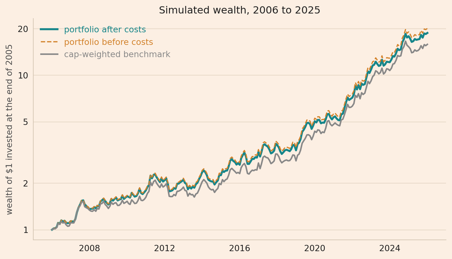
The chart shows the wealth of $1 invested at the end of 2005, on a log scale, where equal distances are equal percentage changes.

import matplotlib.pyplot as plt

TEAL, ORANGE, GREY = "#17868A", "#D2822B", "#888888"
# The site's chart colours: a cream background, a light grid and a pale frame, so every chart
# on the site has the same look.
BG, INK, GRID, SPINE, AXIS_TEXT = "#FCEFE3", "#1f1f1f", "#EADCCC", "#D5C6B4", "#4a4a4a"


def style_chart(figure, axis):
    """Give a finished chart the site's cream background, light grid and pale frame."""
    figure.patch.set_facecolor(BG)
    axis.set_facecolor(BG)
    axis.grid(True, axis="y", color=GRID, lw=1.0)
    axis.set_axisbelow(True)
    for side in ("top", "right"):
        axis.spines[side].set_visible(False)
    for side in ("left", "bottom"):
        axis.spines[side].set_color(SPINE)
    axis.tick_params(axis="both", length=0, colors=INK, pad=6)
    axis.xaxis.label.set_color(AXIS_TEXT)
    axis.yaxis.label.set_color(AXIS_TEXT)
    axis.title.set_color(INK)
    # Each legend entry in the colour of its line; get_legend() returns None without a legend
    legend = axis.get_legend()
    if legend is not None:
        for text, handle in zip(legend.get_texts(), legend.legend_handles):
            text.set_color(handle.get_color())


# figsize is the figure's width and height in inches; lw is the line width, ls="--" dashed
fig, axis = plt.subplots(figsize=(7.6, 4.4))
axis.plot(wealth.index, wealth["after costs"], color=TEAL, lw=2.4, label="portfolio after costs")
axis.plot(wealth.index, wealth["before costs"], color=ORANGE, lw=1.4, ls="--",
          label="portfolio before costs")
axis.plot(wealth.index, wealth["benchmark"], color=GREY, lw=1.8, label="cap-weighted benchmark")
axis.set_yscale("log")        # equal distances are equal percentage changes
axis.set_yticks([1, 2, 5, 10, 20], ["1", "2", "5", "10", "20"])
axis.minorticks_off()
axis.set_ylabel(r"wealth of \$1 invested at the end of 2005")   # \$ prints a dollar sign
axis.set_title("Simulated wealth, 2006 to 2025")
axis.legend(frameon=False, loc="upper left")                   # frameon=False: no box
style_chart(fig, axis)
plt.tight_layout()
# dpi sets the saved image's pixels per inch, and bbox_inches="tight" trims the empty margin
plt.savefig("fi_wealth.png", dpi=140, bbox_inches="tight", facecolor=BG)
plt.show()

years = STUDY_MONTHS / 12
wealth_returns = wealth.pct_change().dropna()    # each month's return; dropna() drops row one
# Turnover per year leaves out the first purchase: the other 79 rebalances span 19.75 years
turnover_per_year = sum(table["trade"].abs().sum() for date, table in rebalances.items()
                        if date != formation_dates[0]) / (years - 0.25)


def annualised_return(wealth_path):
    """The yearly growth rate, in %, that compounds to the final wealth over the 20 years."""
    return (wealth_path.iloc[-1] ** (1 / years) - 1) * 100


def annualised_volatility(monthly):
    """The monthly standard deviation times the square root of 12, in %: the variances of
    independent months add up."""
    return monthly.std() * np.sqrt(12) * 100


# Every ticker with a positive market cap on each formation date, so missing signals cannot
# shrink the benchmark: its percentiles (missing when not eligible), its target weight (0 when
# not selected) and its benchmark weight
at_formation = monthly.loc[monthly["date"].isin(formation_dates) & (monthly["market_cap"] > 0),
                           ["date", "ticker", "market_cap", "sector"]]
at_formation = at_formation.merge(
    scores[["date", "ticker", "value_percentile", "momentum_percentile", "target_weight"]],
    on=["date", "ticker"], how="left")
at_formation["target_weight"] = at_formation["target_weight"].fillna(0.0)
at_formation["cap_weight"] = (at_formation["market_cap"]
                              / at_formation.groupby("date")["market_cap"].transform("sum"))


def weighted_percentile(weight, column):
    """Each date's weighted average percentile over the tickers that have one."""
    has_one = at_formation[column].notna()
    weights = at_formation[weight].where(has_one)
    by_date = at_formation["date"]
    return (weights * at_formation[column]).groupby(by_date).sum() / weights.groupby(by_date).sum()


def holdings_summary(weight):
    """Concentration and tilt of a weight column, averaged over the formation dates."""
    rows = at_formation
    # sort_values then head(10) keeps each date's 10 largest weights
    top_ten = rows.sort_values(weight, ascending=False).groupby("date").head(10)
    measures = pd.DataFrame({
        "effective number of stocks": 1 / (rows[weight] ** 2).groupby(rows["date"]).sum(),
        "weight of the 10 largest (%)": top_ten.groupby("date")[weight].sum() * 100,
        "weighted average value percentile": weighted_percentile(weight, "value_percentile"),
        "weighted average momentum percentile": weighted_percentile(weight, "momentum_percentile"),
        # each sector's total weight per date, then the largest sector of each date
        "largest sector weight (%)":
            rows.groupby(["date", "sector"])[weight].sum().groupby("date").max() * 100,
    })
    return measures.mean()


performance = pd.DataFrame({
    "portfolio": [annualised_return(wealth["before costs"]),
                  annualised_return(wealth["after costs"]),
                  annualised_volatility(wealth_returns["after costs"]), turnover_per_year * 100],
    "benchmark": [annualised_return(wealth["benchmark"]), annualised_return(wealth["benchmark"]),
                  annualised_volatility(wealth_returns["benchmark"]),
                  0.0]},    # the benchmark trades only to reinvest dividends, free in both
    index=["annualised return before costs (%)", "annualised return after costs (%)",
           "annualised volatility (%)", "turnover per year (% of wealth)"])
holding_measures = pd.DataFrame({"portfolio": holdings_summary("target_weight"),
                                 "benchmark": holdings_summary("cap_weight")})
# pd.concat stacks the two tables, the performance rows above the holdings rows
pd.concat([performance, holding_measures]).round(2)

	portfolio	benchmark
annualised return before costs (%)	16.18	14.81
annualised return after costs (%)	15.79	14.81
annualised volatility (%)	16.03	15.88
turnover per year (% of wealth)	332.80	0.00
effective number of stocks	45.02	162.93
weight of the 10 largest (%)	36.77	16.44
weighted average value percentile	0.65	0.36
weighted average momentum percentile	0.75	0.56
largest sector weight (%)	23.82	16.36

The last five rows average the 80 rebalance dates. The portfolio tilts toward both characteristics, with weighted average percentiles above the benchmark’s for value and momentum. It is also more concentrated: its effective number of stocks, \(1/\sum_i w_i^2\), the number of equally weighted stocks with the same sum of squared weights, is 45, against 163, and its largest sector holds about a quarter of its weight, against a sixth for the benchmark. Annualised volatility, the standard deviation of monthly returns scaled to a year, is about 16% for both. Trading costs reduce the portfolio’s annualised return by 0.39 percentage points, to 0.98 points above the benchmark’s. That gap is one outcome of the assumed premium and the random shocks of this simulated path.

This tutorial demonstrates how the portfolio is built and maintained, and its simulated performance depends on the assumptions in the data: the premium, a universe of 500 stocks without listings or delistings, trades at month-end closing prices at exactly 10 basis points, dividends reinvested at no cost, one value ratio and no sector limits.

NoteAdditional checks

The block below checks the timing of both signals and of book equity, that no data from after the formation date enters the weights, the weights at all 80 rebalances, the cap, the drift, the trading costs, the small-cost approximation, the daily data and the safeguards for missing data.

checks = []

# Momentum at t compounds months t-11 to t-1: recompute it from a plain array
row = wide_returns.index.get_loc(EXAMPLE_DATE)
by_hand = np.prod(1 + wide_returns.to_numpy()[row - 11:row], axis=0) - 1
monthly_march = monthly.loc[monthly["date"] == EXAMPLE_DATE].set_index("ticker")
checks.append(("momentum compounds the returns of months t-11 to t-1",
               np.allclose(monthly_march.loc[wide_returns.columns, "momentum"], by_hand)))

# Book equity on each month-end is the latest report published by that date
latest = pd.merge_asof(monthly[["date", "ticker"]].sort_values("date"),
                       fundamentals.sort_values("published"),
                       left_on="date", right_on="published", by="ticker")
latest = latest.set_index(["date", "ticker"])["book_equity"]
checks.append(("month-end book equity is the latest report published by that date",
               latest.sort_index().equals(monthly.set_index(["date", "ticker"])["book_equity"]
                                          .sort_index())))

# The scores and weights at t must not change when the daily data stop at t
known_daily = daily.loc[daily["date"] <= EXAMPLE_DATE]
past_only = add_weights(add_scores(add_characteristics(to_month_ends(known_daily))))
past_march = past_only.loc[past_only["date"] == EXAMPLE_DATE].set_index("ticker")
scores_march = scores.loc[scores["date"] == EXAMPLE_DATE].set_index("ticker")
compared = ["value", "momentum", "score", "target_weight"]
checks.append(("the scores and weights at t use no data from after t",
               past_march[compared].equals(scores_march.loc[past_march.index, compared])))

# Momentum at t must ignore the return of month t itself
changed = to_month_ends(known_daily)
changed.loc[changed["date"] == EXAMPLE_DATE, "return"] += 0.5
changed = add_characteristics(changed)
changed_march = changed.loc[changed["date"] == EXAMPLE_DATE].set_index("ticker")
checks.append(("momentum at t ignores the return of month t",
               np.allclose(changed_march.loc[scores_march.index, "momentum"],
                           scores_march["momentum"])))

# Every target portfolio: 100 tickers, weights that sum to 100%, none negative or above 5%
formation_targets = target_table.loc[formation_dates]
checks.append(("every target holds 100 tickers",
               bool(((formation_targets > 0).sum(axis=1) == N_SELECTED).all())))
checks.append(("every target sums to 100%",
               bool(((formation_targets.sum(axis=1) - 1).abs() < 1e-12).all())))
checks.append(("no target weight is negative or above 5%",
               bool(((formation_targets >= 0) & (formation_targets <= WEIGHT_CAP + 1e-12))
                    .all().all())))

# The cap's excess goes to the other tickers in proportion: one common factor for the uncapped
held = scores_march.loc[scores_march["selected"]]
uncapped = held["target_weight"] < WEIGHT_CAP - 1e-12
factor = held.loc[uncapped, "target_weight"] / held.loc[uncapped, "base_weight"]
checks.append(("the uncapped weights are multiplied by one common factor",
               np.allclose(factor, factor.iloc[0])))

# Drift: the weights before the next rebalance are the targets grown by each ticker's returns
march_target = rebalances[EXAMPLE_DATE]["target"]
growth = (1 + wide_returns.loc[EXAMPLE_DATE:NEXT_REBALANCE].iloc[1:]).prod()
drifted = march_target * growth / (march_target * growth).sum()
checks.append(("the drifted weights are the targets grown by their returns",
               np.allclose(rebalances[NEXT_REBALANCE]["current"], drifted)))

# Costs: the first purchase is a turnover of 100%, and wealth after costs is wealth before costs
# times the product of (1 - 0.001 x turnover) over the rebalances
turnovers = np.array([table["trade"].abs().sum() for table in rebalances.values()])
cost_factor = np.prod(1 - COST_PER_DOLLAR * turnovers)
checks.append(("the first purchase is a turnover of 100%", np.isclose(turnovers[0], 1.0)))
checks.append(("wealth after costs = wealth before costs x product of (1 - 0.001 turnover)",
               np.isclose(wealth["after costs"].iloc[-1],
                          wealth["before costs"].iloc[-1] * cost_factor)))

# The small-cost approximation. The trades are sized on the wealth before costs, 1. Sized on the
# wealth left after costs, W, they would give W = 1 - 0.001 x sum |target x W - current|, and
# applying this formula 20 times, starting from the charged cost, gives W. Is the charged cost
# within 0.1% of the exact cost, 1 - W, at every rebalance?
gaps = []
for table in rebalances.values():
    charged = COST_PER_DOLLAR * table["trade"].abs().sum()
    exact_wealth = 1 - charged
    for repetition in range(20):
        traded = (table["target"] * exact_wealth - table["current"]).abs().sum()
        exact_wealth = 1 - COST_PER_DOLLAR * traded
    gaps.append(abs((1 - exact_wealth) - charged) / (1 - exact_wealth))
checks.append(("sizing the trades on the wealth after costs changes each rebalance's cost "
               "by at most 0.1% of that cost", max(gaps) <= 0.001 + 1e-9))

# The daily data: yesterday's market cap grown by today's total return, minus today's cap, is
# the dividend paid today, which must never be negative
daily_caps = daily.pivot(index="date", columns="ticker", values="market_cap")
daily_returns = daily.pivot(index="date", columns="ticker", values="return")
dividend_yield = (daily_caps.shift(1) * (1 + daily_returns) - daily_caps) / daily_caps.shift(1)
checks.append(("daily market caps, returns and dividends agree: no negative dividend",
               bool((dividend_yield.iloc[1:] > -1e-12).all().all())))

# Missing data. A month with a missing trading day keeps a missing return: S040 lacks two days
# of July 2014 in the copy, so its July return is missing and its June return is not
s040 = gappy.loc[gappy["ticker"] == "S040"].set_index("date")["return"]
checks.append(("a month with a missing trading day keeps a missing return",
               bool(np.isnan(s040.loc["2014-07"]).all() and s040.loc["2014-06"].notna().all())))

# A month with rows but no returns at all stays missing instead of becoming a 0% return
no_returns = daily.loc[daily["ticker"].isin(["S001", "S002"])].copy()
no_returns.loc[no_returns["date"].dt.to_period("M") == "2015-02", "return"] = np.nan
february = to_month_ends(no_returns).set_index("date").loc["2015-02", "return"]
checks.append(("a month with rows but no returns stays missing", bool(february.isna().all())))

# A missing month-end market cap stays missing and is not taken from an earlier day
two = daily.loc[daily["ticker"].isin(["S001", "S002"])].copy()
two.loc[(two["ticker"] == "S001") & (two["date"] == EXAMPLE_DATE), "market_cap"] = np.nan
two_monthly = to_month_ends(two).set_index(["date", "ticker"])
checks.append(("a missing month-end market cap stays missing",
               bool(np.isnan(two_monthly.loc[(EXAMPLE_DATE, "S001"), "market_cap"]))))

# Missing signals leave the benchmark alone: on the example date, the copy with removed inputs
# has the same tickers with a positive market cap, so the same benchmark weights
complete_caps = monthly.loc[monthly["date"] == EXAMPLE_DATE].set_index("ticker")["market_cap"]
gappy_caps = gappy.loc[gappy["date"] == EXAMPLE_DATE].set_index("ticker")["market_cap"]
checks.append(("missing signals leave the benchmark's tickers and weights unchanged",
               gappy_caps.sort_index().equals(complete_caps.sort_index())))


# The safeguards stop the calculation instead of filling in
def raises(function, *arguments):
    """True when calling the function with these arguments raises a ValueError."""
    try:
        function(*arguments)
    except ValueError:
        return True
    return False


some_weights = pd.Series([0.6, 0.4, 0.0], index=["S001", "S002", "S003"])
some_returns = pd.Series([0.01, np.nan, np.nan], index=["S001", "S002", "S003"])
checks.append(("a held ticker without a return stops the backtest",
               raises(check_returns, some_weights, some_returns, "portfolio", EXAMPLE_DATE)
               and not raises(check_returns, some_weights.iloc[[0, 2]],
                              some_returns.iloc[[0, 2]], "portfolio", EXAMPLE_DATE)))
checks.append(("a formation date with fewer than 100 eligible tickers stops the backtest",
               raises(check_candidates, pd.Timestamp("2004-03-31"))
               and not raises(check_candidates, EXAMPLE_DATE)))
no_caps = wide_caps.copy()
no_caps.loc[EXAMPLE_DATE] = 0.0
checks.append(("a month-end without a positive total market cap stops the benchmark",
               raises(benchmark_returns, no_caps, wide_returns, study_dates)))
checks.append(("a repeated ticker-date row stops the monthly conversion",
               raises(to_month_ends, pd.concat([two, two.iloc[:1]]))))

for description, passed in checks:
    print(f"{'passed' if passed else 'FAILED'}: {description}")
assert all(passed for _, passed in checks)

passed: momentum compounds the returns of months t-11 to t-1
passed: month-end book equity is the latest report published by that date
passed: the scores and weights at t use no data from after t
passed: momentum at t ignores the return of month t
passed: every target holds 100 tickers
passed: every target sums to 100%
passed: no target weight is negative or above 5%
passed: the uncapped weights are multiplied by one common factor
passed: the drifted weights are the targets grown by their returns
passed: the first purchase is a turnover of 100%
passed: wealth after costs = wealth before costs x product of (1 - 0.001 turnover)
passed: sizing the trades on the wealth after costs changes each rebalance's cost by at most 0.1% of that cost
passed: daily market caps, returns and dividends agree: no negative dividend
passed: a month with a missing trading day keeps a missing return
passed: a month with rows but no returns stays missing
passed: a missing month-end market cap stays missing
passed: missing signals leave the benchmark's tickers and weights unchanged
passed: a held ticker without a return stops the backtest
passed: a formation date with fewer than 100 eligible tickers stops the backtest
passed: a month-end without a positive total market cap stops the benchmark
passed: a repeated ticker-date row stops the monthly conversion

Read next

• Trading costs more than halved Swedish momentum’s ending value What trading costs did to a momentum portfolio on Swedish stocks.
• Same data, same trading signal, different answer How ordinary choices in building a portfolio can flip its trading decision.

Disclaimer: a teaching example on simulated data, whose returns follow the assumptions in the code. Not investment advice.

Sources: Turan G. Bali, Robert F. Engle and Scott Murray, Empirical Asset Pricing: The Cross Section of Stock Returns (Wiley, 2016), Chapter 5 for weighted portfolio returns and formation timing, Chapter 10 for book-to-market and when fundamentals are public, and Chapter 11 for momentum over months \(t-11\) to \(t-1\). Kenneth French, momentum factor, with prior returns from months 2 to 12 before the holding month. Shaun Fitzgibbons, Jacques Friedman, Lukasz Pomorski and Laura Serban, Long-Only Style Investing: Don’t Just Mix, Integrate, Journal of Investing (2017). S&P Dow Jones Indices, S&P Quality, Value & Momentum Multi-Factor Indices methodology, for weights proportional to market cap times score. Eugene F. Fama and Kenneth R. French, “Common risk factors in the returns on stocks and bonds”, Journal of Financial Economics (1993). The simulation, the 100 stocks, the equal score weights, the 5% cap, quarterly rebalancing and the 10 basis-point cost are assumptions of this tutorial.