import numpy as np
import pandas as pd

SEED = 2026
N_STOCKS = 4000                          # stocks in the market
RISK_FREE = 0.0036                       # r_f, the return on cash, a month
MARKET_MEAN, MARKET_SD = 0.006, 0.045    # M, the shared market return above cash: average, sd
VALUE_MEAN, VALUE_SD = 0.003, 0.030      # V, the shared value return: average, sd
STOCK_SD = 0.08                          # sd of each stock's own random part
ROE_MEAN, ROE_SD = 0.12, 0.08            # return on equity in a fiscal year: average, sd

# The 750 month-ends from July 1963 to December 2025; BMonthEnd() picks each month's last weekday
month_ends = pd.date_range("1963-07-01", "2025-12-31", freq=pd.offsets.BMonthEnd())
# Tickers S0001 to S4000: the numbers 1 to 4,000 as text, filled with zeros to four digits
tickers = "S" + pd.Series(range(1, N_STOCKS + 1)).astype(str).str.zfill(4)

# default_rng(SEED) starts the random number generator, so every run draws the same numbers;
# rng.uniform(a, b, n) draws n numbers equally likely anywhere between a and b, and
# rng.standard_normal(n) draws n normal numbers with an average of 0 and a standard deviation of 1
rng = np.random.default_rng(SEED)
beta = rng.uniform(0.7, 1.3, N_STOCKS)                       # each stock's market beta
cap = 500 * np.exp(1.5 * rng.standard_normal(N_STOCKS))      # market caps, $ millions
book = cap * np.exp(np.log(0.7) + 0.7 * rng.standard_normal(N_STOCKS))     # book equity
published_book = book.copy()        # the book equity of each stock's latest published report

# Each month adds a small table of prices to price_tables, and each March a table of reports
# to report_tables. The first reports, for the fiscal year that ended in December 1962, were
# published at the end of March 1963
price_tables = []
report_tables = [pd.DataFrame({"ticker": tickers, "fiscal_year_end": pd.Timestamp("1962-12-31"),
                               "published": pd.Timestamp("1963-03-29"), "book_equity": book})]

for date in month_ends:
    # The value loading h uses the book-to-market at the previous month-end, from the book
    # equity published by then; rank(pct=True) gives each stock its percentile
    percentile = pd.Series(published_book / cap).rank(pct=True).to_numpy()
    loading = (percentile - 0.5) / 0.7
    market = MARKET_MEAN + MARKET_SD * rng.standard_normal()     # M, the same for every stock
    value = VALUE_MEAN + VALUE_SD * rng.standard_normal()        # V, the same for every stock
    stock_returns = (RISK_FREE + beta * market + loading * value
                     + STOCK_SD * rng.standard_normal(N_STOCKS))
    cap = cap * (1 + stock_returns)
    price_tables.append(pd.DataFrame({"date": date, "ticker": tickers,
                                      "return": stock_returns, "market_cap": cap}))
    if date.month == 12:
        # The fiscal year ends: book equity grows by the year's return on equity
        book = book * (1 + ROE_MEAN + ROE_SD * rng.standard_normal(N_STOCKS))
    if date.month == 3:
        # The report on the year that ended in December is published at the end of March
        published_book = book.copy()
        report_tables.append(pd.DataFrame({"ticker": tickers,
                                           "fiscal_year_end": pd.Timestamp(date.year - 1, 12, 31),
                                           "published": date, "book_equity": book}))

# concat stacks the small tables into one, and ignore_index numbers its rows from 0
prices = pd.concat(price_tables, ignore_index=True)
reports = pd.concat(report_tables, ignore_index=True)Testing a stock characteristic as a factor
Python
Backtesting
Tutorial
Code
How to go from an economic idea about a characteristic to the evidence that it is a factor, in five steps, with value on simulated data.
Part 2 of 3 in a series on stock characteristics and factors: 1. What a straight line can miss about stock returns, 2. Testing a stock characteristic as a factor, 3. How to do factor investing.
Part 1 sorted stocks into groups to measure whether a characteristic predicts next month’s return. A characteristic that predicts returns is not yet a factor. Here, a factor is a return that many stocks share and that explains differences in their average returns.
I pretend not to know whether value predicts returns and test value in five steps on a simulated market in which value is a factor by design. Value stocks, with a high ratio of book equity to market cap, earn 0.34% a month more on average than growth stocks, with a low ratio. This return difference is the value spread. The market does not explain the value spread, and the value spread from one half of the stocks explains the returns of value and growth stocks in the other half.
Simulating the market
The simulated data has the two tables a data vendor delivers, for 4,000 stocks from July 1963 to December 2025: monthly prices, and annual reports with their publication dates.
- Returns. A stock’s monthly return above cash is its market beta times a shared market return, plus its value loading times a shared value return, plus a random part of its own.
- Value loading. The loading increases with the stock’s book-to-market percentile, so value stocks move with the value return and earn its average, and growth stocks move against the value return.
- Calibration. The market return averages 0.6% a month above cash and the value return 0.3%, with standard deviations of 4.5% and 3%, close to Fama and French’s US factors since 1963. Cash pays 0.36% a month.
- Reports. Fiscal years end in December, and reports are published at the end of March.
NoteHow the market is simulated
In month \(t+1\), stock \(i\)’s return is
\[r_{i,t+1} = r_f + \beta_i M_{t+1} + h_{i,t} V_{t+1} + 0.08\,\varepsilon_{i,t+1},\]
where \(r_f = 0.36\%\) is the return on cash, and \(M_{t+1}\) and \(V_{t+1}\) are the shared market return above cash and the shared value return, the same for every stock. Both shared returns are normal (bell-shaped) draws, with averages of 0.6% and 0.3% and standard deviations of 4.5% and 3%; a standard deviation measures how far draws typically are from their average. \(\varepsilon_{i,t+1}\) is a normal draw with an average of 0 and a standard deviation of 1, independent across stocks and months, so each stock’s own random part has a standard deviation of 8% a month. Each stock’s market beta \(\beta_i\) is drawn once, equally likely anywhere between 0.7 and 1.3. The value loading is
\[h_{i,t} = \frac{p_{i,t} - 0.5}{0.7},\]
where \(p_{i,t}\) is the stock’s book-to-market percentile at the end of month \(t\), from the latest published book equity, so the loading runs from about −0.7 to 0.7. Dividing by 0.7 gives the 30% of stocks with the highest book-to-market an average loading 1 higher than the 30% with the lowest.
A stock’s market cap grows with its return, \(C_{i,t+1} = C_{i,t}\,(1 + r_{i,t+1})\), because the firms pay no dividends. Starting market caps are lognormal around $500 million, with a standard deviation of 1.5 in logarithms, and starting book equity is the market cap times a book-to-market ratio, lognormal around 0.7 with a standard deviation of 0.7 in logarithms. Every December, book equity grows by the year’s return on equity, a normal draw with an average of 12% and a standard deviation of 8%, and the report is published at the end of the following March. The first reports, for 1962, count as published in March 1963. Each month ends on its last weekday.
The block below shows the first rows of the two tables, with market cap and book equity in millions of dollars and returns as fractions.
Show the code
# to_string(index=False) prints a table without its row numbers
print(prices.head(3).round({"return": 4, "market_cap": 1}).to_string(index=False))
print()
print(reports.head(3).round({"book_equity": 1}).to_string(index=False))
date ticker return market_cap
1963-07-31 S0001 0.105 22151.3
1963-07-31 S0002 0.098 3327.3
1963-07-31 S0003 -0.056 6102.0
ticker fiscal_year_end published book_equity
S0001 1962-12-31 1963-03-29 4656.5
S0002 1962-12-31 1963-03-29 2480.3
S0003 1962-12-31 1963-03-29 5585.2Step 1. Stating the idea
Value investing buys stocks that are cheap relative to their fundamentals. I measure cheapness by book-to-market, a firm’s book equity divided by its market cap, so a higher book-to-market means a cheaper stock. Stocks with a high book-to-market are value stocks, and stocks with a low one are growth stocks.
The idea is that value stocks earn more than growth stocks. Two reasons are possible: value firms are often in financial distress, so investors may demand a higher return for holding them, or investors overreact to bad news and push value stocks’ prices too low. Before looking at any return, I fix the test: each month, sort the stocks into five groups by book-to-market and compare the next month’s average return of the value stocks in the highest group with that of the growth stocks in the lowest.
Step 2. Measuring the value spread
Step 2 measures whether value stocks earned more than growth stocks. A stock’s book-to-market at the end of month \(t\) is
\[\text{B/M}_{i,t} = \frac{B_{i,t}}{C_{i,t}},\]
where \(B_{i,t}\) is the book equity in the latest report published by then and \(C_{i,t}\) the market cap. Each month, I sort the stocks into five groups, which papers call portfolios, at the 20th, 40th, 60th and 80th percentiles of book-to-market, and a group’s return in month \(t+1\) is the average return of its stocks, as in Part 1:
\[R_{g,t+1} = \frac{1}{N_{g,t}} \sum_{i \in G_{g,t}} r_{i,t+1},\]
where \(G_{g,t}\) is the set of the \(N_{g,t}\) stocks in group \(g\). The value spread is the value stocks’ return minus the growth stocks’ return, \(S_{t+1} = R_{5,t+1} - R_{1,t+1}\), and its t-statistic measures how far its average is from zero in standard errors:
\[t = \frac{\bar S}{s/\sqrt{T}},\]
where \(\bar S\) is the average value spread over the \(T\) months, \(s\) its standard deviation, and \(s/\sqrt{T}\) the standard error of the average when months are independent.
Show the code
# duplicated marks each row whose date and ticker already appeared in an earlier row
if prices.duplicated(["date", "ticker"]).any():
    raise ValueError("a ticker appears twice on one month-end")
# merge_asof gives each row the book equity of the ticker's last report published on or before
# the row's date, and needs both tables sorted by date
panel = pd.merge_asof(prices.sort_values("date"),
                      reports[["ticker", "published", "book_equity"]].sort_values("published"),
                      left_on="date", right_on="published", by="ticker")
panel["book_to_market"] = panel["book_equity"] / panel["market_cap"]
panel = panel.sort_values(["ticker", "date"])
# to_period("M") turns each date into its month, and shift(-1) takes each ticker's next row
panel["month"] = panel["date"].dt.to_period("M")
panel["next_month"] = panel.groupby("ticker")["month"].shift(-1)
panel["next_return"] = panel.groupby("ticker")["return"].shift(-1)
# The last month-end has no next month, so it is left out on purpose. Any other row whose next
# row is not the next month, or has no return, stops the calculation
panel = panel.loc[panel["date"] < panel["date"].max()]
if (panel["next_month"] != panel["month"] + 1).any() or panel["next_return"].isna().any():
    raise ValueError("a stock has no next-month return")
# transform runs qcut within each month-end: qcut cuts book-to-market at its 20th, 40th, 60th
# and 80th percentiles and labels the groups 0 to 4, so adding 1 gives groups 1 to 5
panel["group"] = panel.groupby("date")["book_to_market"].transform(pd.qcut, 5, labels=False) + 1
# Each group's average next-month return; unstack turns the five groups into columns
group_returns = panel.groupby(["date", "group"])["next_return"].mean().unstack("group")
value_spread = group_returns[5] - group_returns[1]           # S: value minus growth
months_used = len(value_spread)                               # T
standard_error = value_spread.std() / np.sqrt(months_used)
print("Average next-month return by book-to-market group, % a month:")
print((group_returns.mean() * 100).round(2).to_string())
print(f"\nValue spread: average {value_spread.mean() * 100:.2f}% a month, standard deviation "
      f"{value_spread.std() * 100:.2f}%, {months_used} months")
print(f"Standard error {standard_error * 100:.3f}%, t-statistic "
      f"{value_spread.mean() / standard_error:.2f}")
Average next-month return by book-to-market group, % a month:
group
1 0.80
2 0.89
3 0.95
4 1.08
5 1.15
Value spread: average 0.34% a month, standard deviation 3.58%, 749 months
Standard error 0.131%, t-statistic 2.63Average next-month return increases from group 1, the growth stocks, to group 5, the value stocks. The value spread averages 0.34% a month over 749 months, with a t-statistic of 2.63. Because 2.63 is above 1.96, the cutoff for the 5% level, the average value spread is statistically different from zero, so value stocks earned more than growth stocks.
Step 3. Testing against the existing factors
Step 3 asks whether the existing factors explain the value spread. The capital asset pricing model (CAPM) has one factor, the market. A regression of the monthly value spread on the market’s monthly return above cash,
\[S_t = \alpha + b\,\text{MKT}_t + e_t,\]
estimates the value spread’s alpha \(\alpha\), the part of its average that the market does not explain, and its market beta \(b\). \(\text{MKT}_t\) is the average return of all the stocks, each with the same weight, minus the return on cash, and \(e_t\) the unexplained part of month \(t\)’s value spread. In this example, I test against the CAPM only. With today’s multifactor models, such as the five factors of Fama and French (2015), we would add each factor’s monthly return to this regression and test whether the alpha is still statistically different from zero. Those five factors already include value, so for value the test would ask whether this version of value adds anything.
Show the code
import statsmodels.api as sm

# MKT: the average return of all the stocks above cash, in each month
market = (panel.groupby("date")["next_return"].mean() - RISK_FREE).rename("market")
# add_constant adds a column of ones, whose coefficient is the intercept, the alpha, and
# cov_type="HAC" gives Newey-West standard errors, which allow for returns related over
# up to 6 months
value_spread_on_market = sm.OLS(value_spread, sm.add_constant(market)).fit(
    cov_type="HAC", cov_kwds={"maxlags": 6})
print(f"Value spread against the market: alpha "
      f"{value_spread_on_market.params['const'] * 100:.2f}% a month, t-statistic "
      f"{value_spread_on_market.tvalues['const']:.2f}")
Value spread against the market: alpha 0.39% a month, t-statistic 2.88The alpha is 0.39% a month, with a t-statistic of 2.88. Because 2.88 is above 1.96, the alpha is statistically different from zero at the 5% level. So, against the CAPM, value is an anomaly: the CAPM does not explain the value spread.
Step 4. Testing the value spread as a factor
Step 3 asked whether the market explains the value spread. Step 4 turns this around and uses the value spread to explain groups of stocks. It asks whether value stocks move together, and whether that shared movement explains their extra average return. If both hold, value is a factor. A value spread built from group 5’s own stocks would correlate with group 5’s return even if value stocks did not move together, so I split the stocks, as Fama and French (1993) did to check their results:
- Split. Each of the 4,000 stocks goes at random into half A or half B, for the whole sample, so each half has value and growth stocks over the same months.
- Half A gives the two factors: its market return above cash, \(\text{MKT}^A_t\), and its value spread, \(S^A_t\), as in Steps 2 and 3.
- Half B gives the returns to explain: its own five book-to-market groups.
I regress each of half B’s groups on half A’s market return alone, as in Step 3, and again with half A’s value spread added:
\[R^B_{g,t} - r_f = \alpha_g + b_g\,\text{MKT}^A_t + h_g\,S^A_t + e_{g,t},\]
where \(h_g\) is the group’s loading on half A’s value spread: how much the group’s return changes when the value spread is 1 percentage point higher and the market’s return is the same. If value is a factor, the loadings increase from the growth stocks of group 1 to the value stocks of group 5, and the alphas become small and not statistically different from zero. \(R^2\) is the share of the variation in the group’s monthly returns that the regression explains.
In this example, I test five groups, each alpha on its own. Fama and French (2015) use sets of 25 groups, such as 25 sorted on size and book-to-market, and test whether all 25 alphas are zero at once with the GRS test of Gibbons, Ross and Shanken (1989).
Show the code
# Each stock joins half A with a chance of 0.5, and half B otherwise. The split has a random
# number generator of its own, with another seed, so its draws are unrelated to the simulation's
split_rng = np.random.default_rng(SEED + 1)
in_half_a = split_rng.uniform(size=N_STOCKS) < 0.5      # True for each stock drawn into half A
tickers_a = tickers[in_half_a]
# isin marks the rows whose ticker is in half A, and ~ swaps True and False
half_a = panel.loc[panel["ticker"].isin(tickers_a)].copy()
half_b = panel.loc[~panel["ticker"].isin(tickers_a)].copy()
# Each half sorts its own stocks into five groups, as in Step 2
half_a["group"] = half_a.groupby("date")["book_to_market"].transform(pd.qcut, 5, labels=False) + 1
half_b["group"] = half_b.groupby("date")["book_to_market"].transform(pd.qcut, 5, labels=False) + 1
groups_a = half_a.groupby(["date", "group"])["next_return"].mean().unstack("group")
groups_b = half_b.groupby(["date", "group"])["next_return"].mean().unstack("group")
# Half A's two factors: its market return above cash and its value spread
factors_a = pd.DataFrame({"market": half_a.groupby("date")["next_return"].mean() - RISK_FREE,
                            "value spread": groups_a[5] - groups_a[1]})

# Each of half B's groups, regressed on half A's market return alone, then with half A's value
# spread added; rsquared is the share of the variation in the group's monthly returns that a
# regression explains
market_rows = []
value_spread_rows = []
for group in range(1, 6):
    return_above_cash = groups_b[group] - RISK_FREE
    market_only = sm.OLS(return_above_cash, sm.add_constant(factors_a["market"])).fit(
        cov_type="HAC", cov_kwds={"maxlags": 6})
    with_value_spread = sm.OLS(return_above_cash, sm.add_constant(factors_a)).fit(
        cov_type="HAC", cov_kwds={"maxlags": 6})
    # t(alpha) is the alpha's t-statistic; se, its standard error, is for the chart
    market_rows.append({"alpha": market_only.params["const"] * 100,
                        "t(alpha)": market_only.tvalues["const"],
                        "R-squared": market_only.rsquared,
                        "se": market_only.bse["const"] * 100})
    value_spread_rows.append({"alpha": with_value_spread.params["const"] * 100,
                              "t(alpha)": with_value_spread.tvalues["const"],
                              "loading h": with_value_spread.params["value spread"],
                              "R-squared": with_value_spread.rsquared,
                              "se": with_value_spread.bse["const"] * 100})
# One table per regression, with one row per group of half B
group_names = ["group 1, growth", "group 2", "group 3", "group 4", "group 5, value"]
market_table = pd.DataFrame(market_rows, index=group_names)
value_spread_table = pd.DataFrame(value_spread_rows, index=group_names)
# drop leaves se out of the printed tables, and replace writes -0.00, a small negative number
# rounded to zero, as 0.00
print("Regression on half A's market return alone (alpha in % a month)")
print(market_table.drop(columns="se").round(2).replace(-0.0, 0.0).to_string())
print("\nRegression on half A's market return and value spread (alpha in % a month)")
print(value_spread_table.drop(columns="se").round(2).replace(-0.0, 0.0).to_string())
Regression on half A's market return alone (alpha in % a month)
alpha t(alpha) R-squared
group 1, growth -0.20 -2.86 0.86
group 2 -0.08 -2.20 0.95
group 3 -0.02 -1.32 0.99
group 4 0.10 2.60 0.95
group 5, value 0.19 2.70 0.84
Regression on half A's market return and value spread (alpha in % a month)
alpha t(alpha) loading h R-squared
group 1, growth -0.01 -0.41 -0.50 0.99
group 2 0.02 0.94 -0.25 0.99
group 3 -0.02 -1.31 0.00 0.99
group 4 0.00 -0.06 0.25 0.99
group 5, value -0.01 -0.40 0.50 0.99Take group 5, the value stocks. Against half A’s market return alone, its alpha is 0.19% a month, with a t-statistic of 2.70, so the alpha is statistically different from zero. With half A’s value spread added, its loading is 0.50: a value spread 1 percentage point higher goes with a group 5 return 0.50 points higher. Its alpha is then −0.01%, with a t-statistic of −0.40, so the alpha is small and no longer statistically different from zero, and its \(R^2\) increases from 0.84 to 0.99. Across the groups, the loadings increase from −0.50 for group 1 to 0.50 for group 5. The chart compares the alphas. Each grey line is a 95% confidence interval: across repeated samples, 95% of such intervals contain the true alpha.
Show the chart code
import matplotlib.pyplot as plt

RED, TEAL, GREY = "#C0392B", "#17868A", "#888888"
# The site's chart colours: a cream background, dark text, a light grid and a pale frame, so every
# chart on the site has the same look
BG, INK, GRID, SPINE, AXIS_TEXT = "#FCEFE3", "#1f1f1f", "#EADCCC", "#D5C6B4", "#4a4a4a"


# figsize is the figure's width and height in inches
fig, axis = plt.subplots(figsize=(7.6, 4.4))
positions = np.arange(1, 6)                      # one position per group, 1 to 5
# Teal bars, left of each group: the alphas against the market alone. width is each bar's
# width, and label is its legend text
axis.bar(positions - 0.19, market_table["alpha"], width=0.38, color=TEAL,
         label="against the market")
# errorbar draws each 95% confidence interval, the alpha plus or minus 1.96 standard errors;
# fmt="none" draws the lines without markers, and lw is the line width
axis.errorbar(positions - 0.19, market_table["alpha"], yerr=1.96 * market_table["se"],
              fmt="none", ecolor=GREY, lw=1.2)
# Red bars, right of each group: the alphas with half A's value spread added
axis.bar(positions + 0.19, value_spread_table["alpha"], width=0.38, color=RED,
         label="against the market and the value spread")
axis.errorbar(positions + 0.19, value_spread_table["alpha"], yerr=1.96 * value_spread_table["se"],
              fmt="none", ecolor=GREY, lw=1.2)
axis.axhline(0, color=SPINE, lw=1)               # the zero line
axis.set_xticks(positions, ["group 1\ngrowth", "group 2", "group 3", "group 4", "group 5\nvalue"])
axis.set_ylabel("alpha, % a month", color=AXIS_TEXT)
axis.set_title("Half B's alphas, before and after adding half A's value spread", color=INK)
# frameon=False draws no box around the legend, and labelcolor="linecolor" writes each entry
# in the colour of its bars
axis.legend(frameon=False, loc="upper left", labelcolor="linecolor")
# The site's look: a cream background, a light grid behind the bars, a pale frame on the left
# and bottom only, and no tick marks
fig.patch.set_facecolor(BG)
axis.set_facecolor(BG)
axis.grid(True, axis="y", color=GRID, lw=1.0)
axis.set_axisbelow(True)
axis.spines[["top", "right"]].set_visible(False)
axis.spines[["left", "bottom"]].set_color(SPINE)
axis.tick_params(axis="both", length=0, colors=INK, pad=6)

plt.tight_layout()   # fits the labels inside the figure
# dpi sets the saved image's pixels per inch, and bbox_inches="tight" trims the empty margin
plt.savefig("tf_alphas.png", dpi=140, bbox_inches="tight", facecolor=BG)
plt.show()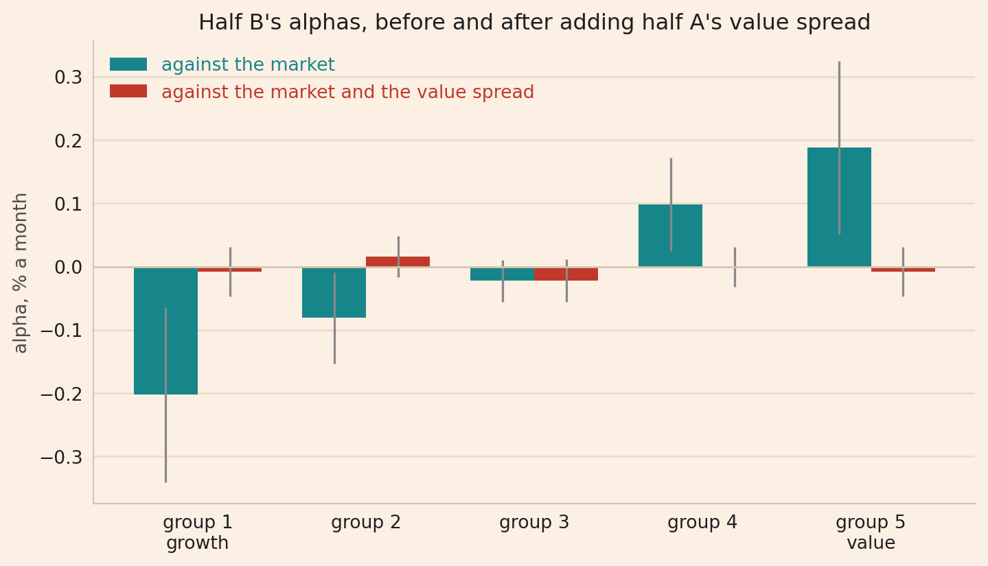
Against the market alone, the teal alphas increase from −0.20% a month for group 1 to 0.19% for group 5. With half A’s value spread added, the red alphas are between −0.02% and 0.02%, and every interval contains zero. So, adding half A’s value spread leaves small alphas for half B’s value and growth stocks, as expected for a factor.
Step 5. Checking new data
Step 5 repeats the same test on new data, such as later years or other countries. A new simulated sample would follow the same assumptions, so this step needs real data, where predictors earn less after they are published (McLean and Pontiff, 2016).
Limitations
Step 4 sorts the groups on the characteristic being tested. A factor should also explain groups sorted in other ways, such as by size or by industry (Lewellen, Nagel and Shanken, 2010).
The tests do not show why value stocks earn more. A reward for risk and a mispricing that affects many value stocks at once can produce the same loadings and alphas.
The 5% cutoff assumes one test, fixed in advance. A characteristic picked from many tested ones needs a t-statistic of about 3 or more, because some of the tested ones exceed 1.96 by chance (Harvey, Liu and Zhu, 2016).
Conclusion
In this simulated market, value passes the first four steps: the value spread averages 0.34% a month (t = 2.63), the CAPM does not explain it, and the value spread from one half of the stocks explains the returns of value and growth stocks in the other half. The fifth step needs real data.
The takeaway is that predicting returns makes a characteristic a candidate. Adding it as a factor needs two more results: the return of its highest group minus its lowest group has an alpha against the factors already in use, and that return explains the average returns of the many stocks that share it. Part 3 builds a portfolio on value and momentum as factors.
Read next
- How to do factor investing Value and momentum in a long-only portfolio, with rebalancing and trading costs.
- In a market with no edge, tuning against the hold-out produced a Sharpe ratio of 2.8 Why a test on new data has to be run once.
Disclaimer: a teaching example on simulated data, whose returns follow the assumptions in the code. Not investment advice.
Sources: Eugene F. Fama and Kenneth R. French, “Common risk factors in the returns on stocks and bonds”, Journal of Financial Economics 33(1), 3-56 (1993), and “A five-factor asset pricing model”, Journal of Financial Economics 116(1), 1-22 (2015). Michael R. Gibbons, Stephen A. Ross and Jay Shanken, “A test of the efficiency of a given portfolio”, Econometrica 57(5), 1121-1152 (1989). Campbell R. Harvey, Yan Liu and Heqing Zhu, “… and the Cross-Section of Expected Returns”, Review of Financial Studies 29(1), 5-68 (2016). Jonathan Lewellen, Stefan Nagel and Jay Shanken, “A skeptical appraisal of asset pricing tests”, Journal of Financial Economics 96(2), 175-194 (2010). R. David McLean and Jeffrey Pontiff, “Does academic research destroy stock return predictability?”, Journal of Finance 71(1), 5-32 (2016). John H. Cochrane, Asset Pricing, revised edition (Princeton University Press, 2005), chapters 12 and 20. Kenneth French’s data library.