Does your backtested Sharpe ratio show a real edge?

On a simulated market built to contain no edge, a search across 216 strategies returns a winner with a Sharpe ratio of 0.72. Bootstrapping shows how much of that is precision and how much is the search itself.

A backtest gives one Sharpe ratio, and that number carries uncertainty. Part of it comes from the properties of financial data, and part from my own choices. In this post, I show how bootstrapping can reduce some of the uncertainty surrounding a backtested Sharpe ratio. It does not resolve every uncertainty in a trading strategy, so I treat it as a starting point.

To make the size of the problem visible, I run the whole exercise on a market I build myself, where nothing can be predicted. A search across 216 strategies still finds a winner with a Sharpe ratio of 0.72.

What bootstrapping does

That one number comes from one historical path, and that path is only one of many the market could have taken. Under a different sequence of returns, the Sharpe ratio would also have been different.

Bootstrapping uses the data I already have to simulate those alternative paths. I resample the observed returns with replacement and in blocks, so that some of the day-to-day dependence remains intact. I then recompute the Sharpe ratio for each resampled series.

Repeating this thousands of times turns one estimate into a distribution. The spread of that distribution measures the uncertainty that the original Sharpe ratio alone does not show.

A market with no edge

To test the approach, I simulate a market with no genuine edge, so any pattern a strategy finds is noise.

I simulate 40 stocks over 3,024 trading days, or about twelve years. Each is driven by a common market factor and its own noise. The factor has clustered volatility, which is why I resample in blocks of consecutive days. The simulation contains no momentum, reversal, or low-volatility effect.

import numpy as np
import pandas as pd

def simulate_panel(n_stocks=40, n_days=3024, momentum_edge=0.0, seed=7):
    rng   = np.random.default_rng(seed)
    dates = pd.bdate_range("2014-01-02", periods=n_days)
    beta  = rng.uniform(0.6, 1.4, n_stocks)      # exposure to the market factor
    idio  = rng.uniform(0.012, 0.022, n_stocks)  # stock-specific daily vol

    h, mkt, eps = np.empty(n_days), np.empty(n_days), rng.standard_normal(n_days)
    h[0] = 0.01 ** 2
    for t in range(n_days):                      # GARCH-like market: volatility clusters
        if t:
            h[t] = 0.01**2 * 0.05 + 0.90 * h[t-1] + 0.05 * mkt[t-1]**2
        mkt[t] = np.sqrt(h[t]) * eps[t]              # zero-mean factor: no premium to earn

    R = np.zeros((n_days, n_stocks))
    for t in range(n_days):
        drift = np.zeros(n_stocks)
        if momentum_edge and t > 252:            # off by default, so there is no edge to find
            past  = R[t-252:t].sum(axis=0)
            drift = momentum_edge * (past - past.mean()) / (past.std() + 1e-12)
        R[t] = drift + beta * mkt[t] + idio * rng.standard_normal(n_stocks)

    return pd.DataFrame(R, index=dates, columns=[f"S{i:02d}" for i in range(n_stocks)])

returns = simulate_panel()                       # momentum_edge = 0
print(f"{returns.shape[1]} stocks x {returns.shape[0]} trading days, "
      f"{returns.index[0].date()} to {returns.index[-1].date()}")

40 stocks x 3024 trading days, 2014-01-02 to 2025-08-05

Searching for the best strategy

I run 216 strategies on the same simulated market: three signal families, six lookback windows, four portfolio sizes, and three trading lags.

Each is dollar-neutral, buying the strongest stocks, selling the weakest, and rebalancing monthly. Because the stocks have different betas, some market-factor exposure remains. The factor is zero-mean, so no strategy has an expected edge by construction.

LOOKBACKS, HOLDINGS, SKIPS = [21, 42, 63, 126, 189, 252], [3, 5, 8, 12], [1, 5, 21]

def long_short(signal, n_hold, reb):
    longs  = ((signal.rank(axis=1, ascending=False) <= n_hold) & signal.notna()).astype(float)
    shorts = ((signal.rank(axis=1, ascending=True)  <= n_hold) & signal.notna()).astype(float)
    w = (longs.div(longs.sum(axis=1).replace(0, np.nan), axis=0)
         - shorts.div(shorts.sum(axis=1).replace(0, np.nan), axis=0))
    return w.where(reb).ffill()                  # set on rebalance days, hold in between, missing until active

def build_grid(returns):
    logret = np.log1p(returns)
    month  = returns.index.to_series().groupby([returns.index.year, returns.index.month])
    first  = month.transform("first") == returns.index
    reb    = pd.DataFrame(np.repeat(first.values[:, None], returns.shape[1], axis=1),
                          index=returns.index, columns=returns.columns)
    out = {}
    for lb in LOOKBACKS:
        trail = logret.rolling(lb).sum()
        rvol  = returns.rolling(lb).std()
        for sk in SKIPS:
            for nh in HOLDINGS:
                sigs = {"mom":  trail.shift(sk),                                  # buy the winners
                        "rev": -logret.rolling(max(lb // 3, 5)).sum().shift(sk),  # buy the losers
                        "lvol": -rvol.shift(sk)}                                  # buy the low-volatility stocks
                for name, sig in sigs.items():
                    w = long_short(sig, nh, reb)
                    out[f"{name}_lb{lb}_n{nh}_sk{sk}"] = (w.shift(1) * returns).sum(axis=1, min_count=1)
    return pd.DataFrame(out).dropna(how="any")    # keep only days on which every strategy is active

def sharpe(x, axis=0):
    x = np.asarray(x)
    return x.mean(axis=axis) / x.std(axis=axis, ddof=1) * np.sqrt(252)

strats   = build_grid(returns)
observed = pd.Series(sharpe(strats.values), index=strats.columns)
winner   = observed.idxmax()

print(f"{strats.shape[1]} candidates over {strats.shape[0]} common days")
print(f"grid Sharpe   min {observed.min():.2f} | median {observed.median():.2f} | "
      f"90th {observed.quantile(0.90):.2f} | max {observed.max():.2f}")
print(f"winner        {winner}   Sharpe {observed[winner]:.2f}")

216 candidates over 2741 common days
grid Sharpe   min -0.68 | median 0.08 | 90th 0.45 | max 0.72
winner        rev_lb21_n3_sk1   Sharpe 0.72

Every signal is lagged by at least one day, and .shift(1) applies today’s return to yesterday’s holdings. No strategy uses information that was unavailable when the position was formed.

The search selects a 21-day reversal strategy holding three stocks on each side, with a Sharpe ratio of 0.72 over nearly eleven years. The strategy looks good and means nothing here: in this simulation, past returns contain no information about future expected returns, so its performance comes from chance.

Method 1: How precise is that 0.72?

With the winner fixed, I resample its daily returns in blocks and recompute its Sharpe ratio thousands of times.

I use the stationary bootstrap of Politis and Romano (1994), which draws blocks of varying length and lets them wrap around the series. This preserves short-run dependence while giving every day the same chance of being selected.

def block_indices(n, B, mean_block, seed=101):
    """B resampled day-orderings of length n, drawn in blocks of ~mean_block days."""
    rng, p = np.random.default_rng(seed), 1.0 / mean_block
    idx = np.empty((B, n), dtype=np.int32)
    idx[:, 0] = rng.integers(0, n, B)
    for t in range(1, n):
        new = rng.random(B) < p                  # start a fresh block...
        idx[:, t] = np.where(new, rng.integers(0, n, B),
                             (idx[:, t-1] + 1) % n)   # ...or continue the current one, wrapping at the end
    return idx

def bootstrap_sharpes(R, idx):
    """Sharpe of every column of R, for every resample in idx."""
    B, n   = idx.shape
    counts = np.zeros((B, n))
    for b in range(B):
        counts[b] = np.bincount(idx[b], minlength=n)   # how often each day was drawn
    s1, s2 = counts @ R, counts @ R**2                 # sums and sums of squares, per draw, per strategy
    mean   = s1 / n
    var    = (s2 - n * mean**2) / (n - 1)
    return mean / np.sqrt(var) * np.sqrt(252)

B, MEAN_BLOCK = 5_000, 21
idx = block_indices(strats.shape[0], B, MEAN_BLOCK)

m1     = bootstrap_sharpes(strats[[winner]].values, idx).ravel()
lo, hi = np.percentile(m1, [2.5, 97.5])

print(f"observed Sharpe   {observed[winner]:.2f}")
print(f"bootstrap se      {m1.std():.2f}")
print(f"95% interval      [{lo:.2f}, {hi:.2f}]")
print(f"P(Sharpe <= 0)    {(m1 <= 0).mean():.1%}")

observed Sharpe   0.72
bootstrap se      0.30
95% interval      [0.14, 1.31]
P(Sharpe <= 0)    0.7%

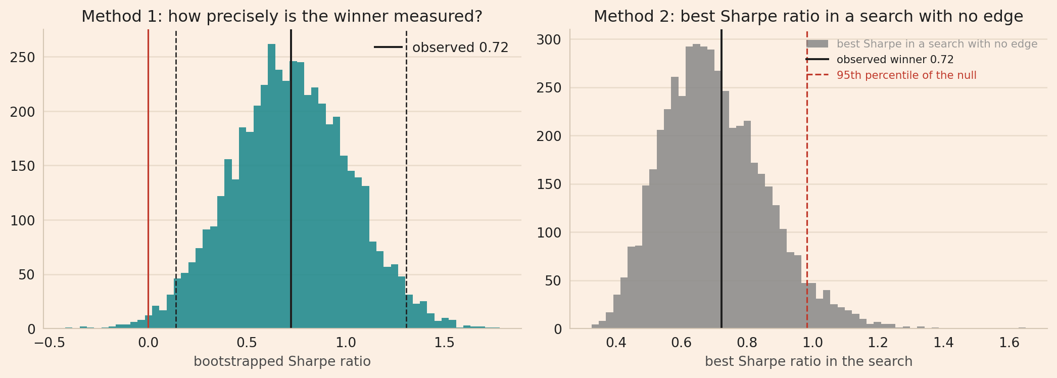
The distribution is centred near 0.72 and it is wide. The 95% interval runs from 0.14 to 1.31, with a standard error of 0.30, and it remains similar across reasonable block lengths. Even with eleven years of daily data, the Sharpe ratio is estimated to roughly one significant figure. It is a noisy measurement.

There is a catch. The interval remains above zero, and fewer than one bootstrap sample in a hundred produces a Sharpe ratio at or below zero. Although the strategy appears significant by a conventional test, the simulation contains no predictable expected returns, so the result is still produced by chance. Method 1 measures estimation uncertainty and does not account for how the strategy was selected.

If the resampling is new to you, Lesson 36 builds the same idea on a single return series, and Lesson 33 covers the Sharpe ratio itself.

Method 2: Is the winner better than luck?

The 0.72 is the highest Sharpe ratio among 216 strategies. The best result from a large search can look strong even when none of the strategies has an edge.

Method 1 looks only at the selected strategy. It therefore ignores that the strategy was chosen because it had the highest Sharpe ratio among 216 alternatives.

Method 2 recreates the entire search after removing the average return from every strategy. Each strategy then has a mean return of zero, while its volatility and co-movement with the others remain intact. I resample the same days for all 216 strategies and record the highest Sharpe ratio in each resampled search.

Repeating this thousands of times shows how high the winning Sharpe ratio can rise from searching alone. I then compare the observed 0.72 with that distribution.

null_panel     = strats - strats.mean()          # every candidate now has zero mean return
null_grid      = bootstrap_sharpes(null_panel.values, idx)   # (5000 draws x 216 candidates)
best_of_search = null_grid.max(axis=1)           # keep only the winner of each simulated search

p_value = (1 + (best_of_search >= observed[winner]).sum()) / (B + 1)

print(f"best Sharpe from a search with no edge:")
print(f"  median {np.median(best_of_search):.2f} | 90th {np.percentile(best_of_search, 90):.2f} "
      f"| 95th {np.percentile(best_of_search, 95):.2f} | max {best_of_search.max():.2f}")
print(f"our winner   {observed[winner]:.2f}")
print(f"p-value      {p_value:.3f}   (beats {(observed[winner] > best_of_search).mean():.0%} of noise searches)")

best Sharpe from a search with no edge:
  median 0.69 | 90th 0.91 | 95th 0.98 | max 1.65
our winner   0.72
p-value      0.407   (beats 59% of noise searches)

A search across 216 no-edge strategies produces a median winning Sharpe ratio of 0.69. In 41% of the bootstrap samples, the highest Sharpe ratio exceeds the observed 0.72, giving a p-value of 0.41. So, once the full search is accounted for, the 0.72 is ordinary.

The two methods answer different questions. Method 1 asks how precisely the winner’s Sharpe ratio is estimated. The answer is imprecisely, although the interval remains above zero. Method 2 asks whether 0.72 is unusual after searching across 216 strategies. The answer is no.

import matplotlib.pyplot as plt

fig, ax = plt.subplots(1, 2, figsize=(11, 4))

ax[0].hist(m1, bins=60, color="#4C72B0", alpha=.85)
ax[0].axvline(observed[winner], color="k", lw=1.5, label=f"observed {observed[winner]:.2f}")
ax[0].axvline(lo, color="k", ls="--", lw=1)
ax[0].axvline(hi, color="k", ls="--", lw=1)
ax[0].axvline(0, color="#C44E52", lw=1.2)
ax[0].set_title("Method 1: how precisely is the winner measured?")
ax[0].set_xlabel("bootstrapped Sharpe ratio")
ax[0].legend(frameon=False)

ax[1].hist(best_of_search, bins=60, color="#999999", alpha=.85,
           label="best Sharpe in a search with no edge")
ax[1].axvline(observed[winner], color="k", lw=1.5, label=f"observed winner {observed[winner]:.2f}")
ax[1].axvline(np.percentile(best_of_search, 95), color="#C44E52", ls="--", lw=1.2,
              label="95th percentile of the null")
ax[1].set_title("Method 2: how good is the winner when nothing works?")
ax[1].set_xlabel("best Sharpe ratio in the search")
ax[1].legend(frameon=False, fontsize=8)

plt.tight_layout()
plt.savefig("sharpe_uncertainty.png", dpi=120, bbox_inches="tight")
plt.show()

On the left, Method 1 places the winner’s Sharpe ratio well above zero. On the right, Method 2 places the same 0.72 near the centre of the Sharpe ratios produced by searches in which every strategy has a mean return of zero.

A check with a real edge

The first simulation shows that Method 2 can reject a winner produced by chance. I now test whether it can also identify a genuine effect. I repeat the analysis after adding momentum to the simulated returns, so that past winners have higher expected returns.

real     = build_grid(simulate_panel(momentum_edge=0.0003))     # a genuine edge, this time
obs_r    = pd.Series(sharpe(real.values), index=real.columns)
win_r    = obs_r.idxmax()
idx_r    = block_indices(real.shape[0], B, MEAN_BLOCK)

m1_r     = bootstrap_sharpes(real[[win_r]].values, idx_r).ravel()
null_r   = bootstrap_sharpes((real - real.mean()).values, idx_r).max(axis=1)
p_r      = (1 + (null_r >= obs_r[win_r]).sum()) / (B + 1)

print(f"winner        {win_r}   Sharpe {obs_r[win_r]:.2f}")
print(f"Method 1      95% interval [{np.percentile(m1_r, 2.5):.2f}, {np.percentile(m1_r, 97.5):.2f}]")
print(f"Method 2      null median {np.median(null_r):.2f}, 95th {np.percentile(null_r, 95):.2f} "
      f"->  p = {p_r:.4f}")

winner        mom_lb252_n12_sk5   Sharpe 1.36
Method 1      95% interval [0.75, 1.95]
Method 2      null median 0.69, 95th 1.00 ->  p = 0.0008

The search recovers the planted effect. The winner is a 252-day momentum strategy with a Sharpe ratio of 1.36 and a p-value of 0.0008. The null distribution barely changes, with a median near 0.69. The earlier Sharpe ratio of 0.72 falls inside the range that the search can produce by chance. The new Sharpe ratio of 1.36 falls well outside it.

What bootstrapping does not fix

Method 2 gives a p-value and leaves the selection bias in the reported Sharpe ratio. The 1.36 is still the highest result among 216 strategies, so it is likely to overstate the strategy’s performance outside this sample.

The result also depends on including the full search. Every specification tested and later discarded still counts as a trial. Omitting them narrows the null distribution and makes the winner appear more unusual.

Finally, both methods resample the history already observed. They do not show how the strategy would perform after trading costs or under a future market that behaves differently. Deduct costs before running the test. Measure returns against an appropriate benchmark where one applies. The strategies here are dollar-neutral, which removes net capital exposure, and because the betas differ, some market-factor exposure can remain.

What it means

A backtested Sharpe ratio carries two kinds of uncertainty. Method 1 measures how much the estimate could change under another sequence of days. Method 2 asks whether the winning Sharpe ratio is unusual once the full search is taken into account.

The takeaway is that the two together reduce the risk of mistaking sampling noise or strategy selection for a genuine edge.

Read next

• When out of sample stops being out of sample The sequel: how a single strategy, tuned against a hold-out, inflates it without any formal grid.
• Why a model with no predictive power can score 90% accuracy Another way validation fails, through outcomes that overlap in time.

Disclaimer: This is a teaching example using synthetic data. The returns are generated, and the first simulation contains no predictable expected returns by construction. This is not investment advice.