import numpy as np
import itertools
import matplotlib.pyplot as plt

RED, TEAL, GREY = "#C0392B", "#17868A", "#888888"
# The site's chart colours: a cream background, a light grid and a pale frame, so every chart
# on the site has the same look.
BG, INK, GRID, SPINE, AXIS_TEXT = "#FCEFE3", "#1f1f1f", "#EADCCC", "#D5C6B4", "#4a4a4a"

MONTHS = 180                 # the length of the simulated history
STOCKS = 300                 # how many stocks the simulated market holds
SIGNAL_PERSISTENCE = 0.90    # how much of last month's signal is kept in this month
MONTHS_IN_YEAR = 12
EDGE = 0.0014
CUTOFF = 0.6


def style_chart(figure, axis):
    """Give a finished chart the site's cream background, light grid and pale frame."""
    figure.patch.set_facecolor(BG)
    axis.set_facecolor(BG)
    axis.grid(True, axis="y", color=GRID, lw=1.0)
    axis.set_axisbelow(True)
    for side in ("top", "right"):
        axis.spines[side].set_visible(False)
    for side in ("left", "bottom"):
        axis.spines[side].set_color(SPINE)
    axis.tick_params(axis="both", length=0, colors=INK, pad=6)
    axis.xaxis.label.set_color(AXIS_TEXT)
    axis.yaxis.label.set_color(AXIS_TEXT)
    axis.title.set_color(INK)
    # Each legend entry in the colour of what it labels: a line's colour or a bar's fill.
    # get_legend() returns None when the chart has no legend.
    legend = axis.get_legend()
    if legend is not None:
        for text, handle in zip(legend.get_texts(), legend.legend_handles):
            if hasattr(handle, "get_color"):
                text.set_color(handle.get_color())
            else:
                text.set_color(handle.get_facecolor())


def make_panel(seed, edge=EDGE):
    """Simulate one market and return the size, the signal and the return of every stock.

    The size array holds one number per stock. The signal and return arrays both hold one
    row per month and one column per stock.
    """
    random_generator = np.random.default_rng(seed)

    # Size is the exponential of a normal draw, which gives a long right tail, so a few
    # stocks end up far larger than the rest the way they do in a real market.
    stock_size = np.exp(random_generator.normal(0, 1.0, STOCKS))

    # The signal persists from month to month. Each month keeps SIGNAL_PERSISTENCE of
    # last month's value and adds fresh noise on top. The square root sizes that noise so
    # the signal keeps a standard deviation of one rather than growing over the sample.
    noise_scale = np.sqrt(1 - SIGNAL_PERSISTENCE**2)
    signal = np.empty((MONTHS, STOCKS))
    signal[0] = random_generator.normal(0, 1, STOCKS)
    for month in range(1, MONTHS):
        carried_over = SIGNAL_PERSISTENCE * signal[month - 1]
        fresh_noise = noise_scale * random_generator.normal(0, 1, STOCKS)
        signal[month] = carried_over + fresh_noise

    # Returns start as pure noise, and the edge is then added on top. Row 1 onwards gets
    # the signal from the row above, so this month's return pays off last month's signal.
    stock_return = random_generator.normal(0, 0.06, (MONTHS, STOCKS))
    stock_return[1:] += edge * signal[:-1]
    return stock_size, signal, stock_return


# One dataset, from a fixed seed, so the post reports the same numbers on every render.
panel_size, panel_signal, panel_return = make_panel(0)Same data, same trading signal, different answer
Python
Backtesting
Tutorial
Code
On simulated data with a real edge, at least one of ten ordinary changes in how the portfolio is built flips the trading decision in 79% of datasets.

Menkveld and co-authors (2024) gave 164 research teams the same data, 17 years of trading in EuroStoxx 50 futures, and the same six hypotheses to test. The teams came back with different answers. For one hypothesis, 125 of the 164 teams found a statistically significant result, one unlikely to arise by chance alone. For another hypothesis, six teams did. The authors call the variation across teams the nonstandard error: the uncertainty that comes from who runs the analysis, on top of the uncertainty that comes from the data. In their experiment, the two uncertainties were about the same size.
The variation has a plain source: each team turned each hypothesis into its own measure, choosing what to compute, how often to sample the data and what to do with outliers.
Menkveld’s teams tested hypotheses. My question is whether the answers also differ when the output is a trading strategy’s backtest. As far as I know, no one has given 164 quants the same data and collected their backtests, so I show the mechanism on a simulated market where I know the truth: in 300 stocks, a signal predicts returns. I build one long-short portfolio on the signal, buying the stocks with the highest signal and selling short, betting against, those with the lowest. Then I change how I build it, one choice at a time, as another quant might, and measure how the backtest’s result changes.
The issue is that a backtest reports one build of a strategy, one set of choices about how to construct its portfolio. On one simulated dataset, the 576 builds of the same signal report annual returns from -1.6% to +6.3%, and ordinary choices about the build decide whether I would trade the strategy at all.
Simulating the data
- Market: 300 simulated stocks over 180 months.
- Signal: one number per stock that moves slowly, and, in truth, last month’s value predicts this month’s return.
- Portfolio: long the stocks with the highest signal, short the lowest, with the holdings reset each month.
- Costs: charged on turnover, the share of the portfolio traded each month, in basis points, where one basis point is 0.01%.
- Decision: I trade the portfolio if its Sharpe ratio is above 0.6, a cutoff I vary later. The Sharpe ratio is \(\sqrt{12}\,\bar R/s\), the annual return divided by the annual volatility, where \(\bar R\) is the average monthly return and \(s\) the standard deviation of the monthly returns, a measure of how far they typically are from their average.
In the simulation, stock \(i\)’s signal and return in month \(t\) are
\[s_{i,t} = 0.9\,s_{i,t-1} + \sqrt{1 - 0.9^2}\;u_{i,t}, \qquad r_{i,t} = 0.0014\,s_{i,t-1} + 0.06\,\varepsilon_{i,t},\]
where \(u_{i,t}\) and \(\varepsilon_{i,t}\) are draws from the standard normal distribution, which is bell-shaped with a mean of 0 and a standard deviation of 1, independent across stocks and months; the first month’s signals are standard normal draws too. The signal keeps 90% of last month’s value, and the factor \(\sqrt{1 - 0.9^2}\) keeps its variance, the squared standard deviation, at 1: \(0.9^2 + (1 - 0.9^2) = 1\). A stock whose signal was one standard deviation above average last month earns 0.14 percentage points a month more in expectation, against noise with a standard deviation of 6% a month. Each stock also has a size, \(e\) raised to a standard normal draw, so a few stocks are far larger than the rest. The 0.9, the 0.14 percentage points, the 6% and the spread of sizes are assumptions. The box below has the code that simulates the market.
NoteHow the market is simulated
The block below sets the constants, simulates the market with make_panel, and defines the chart style used later.
Building the portfolio
Building the portfolio takes eight choices: how far back to average the signal, whether to trim extreme returns, which stocks to drop, how to weight the rest, how many groups to sort them into, how long to wait after the signal, how often to rebalance, and what one trade costs. Whatever the choices, each month the portfolio earns
\[R_t = \sum_i w_{i,t}\, r_{i,t} - c \sum_i \lvert w_{i,t} - w_{i,t-1} \rvert,\]
where \(w_{i,t}\) is the weight on stock \(i\), positive for the stocks bought and negative for those sold short, with the long weights adding up to 1 and the short weights to −1. The sum of the absolute weight changes is the turnover, and \(c\), the cost per unit traded, is 10 basis points in the plain build, the starting set of choices described below. None of the eight choices follows from the signal. Seven change the portfolio, and trimming changes only how its returns are measured: trimming at 1% caps each month’s stock returns at that month’s 1st and 99th percentiles, while the portfolio still earns the untrimmed returns.
def build(stock_size, signal, stock_return, window, winsor, liquidity, weighting,
          groups, lag, rebalance, cost_bps):
    """Run one long-short portfolio and return what it earned in every month.

    The eight arguments after the three data arrays are the eight choices this post is
    about, and the return is one net number per traded month.
    """
    # liquidity is the fraction of the smallest stocks to leave out. np.quantile reads off
    # the size at that fraction, and the comparison gives an array of True and
    # False. At liquidity 0.0 the quantile is the smallest size of all, so every stock is kept.
    size_cutoff = np.quantile(stock_size, liquidity)
    keep = stock_size >= size_cutoff

    # A True and False array inside the brackets picks the columns where it is True, and
    # that kind of indexing already hands back a new array rather than a view. The .copy()
    # says so in the code, because the averaging below writes into signal_kept.
    signal_kept = signal[:, keep].copy()
    return_kept = stock_return[:, keep]
    size_kept = stock_size[keep]
    n_kept = signal_kept.shape[1]     # shape is (months, stocks), so [1] counts the stocks

    if window > 1:
        # A trailing average of the last `window` months of the signal. Adding each window
        # up on its own would redo most of the work, so cumsum runs one running total down
        # each column, and the sum of any window is then one running total minus an earlier
        # one. The row of zeros on top gives the first window something to subtract from.
        running_total = np.vstack([np.zeros((1, n_kept)), np.cumsum(signal_kept, axis=0)])
        window_sum = running_total[window:] - running_total[:-window]
        signal_kept[window - 1:] = window_sum / window

    if winsor > 0:
        # Trimming pulls the most extreme stock returns of each month back to a percentile,
        # so that one extreme return cannot determine the result. axis=1 computes across the stocks
        # within a month, and keepdims holds on to the month axis so that the cutoffs align
        # row by row when np.clip applies them.
        low_cut, high_cut = np.percentile(return_kept, [winsor, 100 - winsor],
                                          axis=1, keepdims=True)
        return_kept = np.clip(return_kept, low_cut, high_cut)

    # The first month that can be traded needs the averaging window filled and the lag
    # served, and both are counted from the start of the sample.
    first_month = lag + window - 1
    n_per_side = max(1, n_kept // groups)   # 5 groups puts a quintile on each side

    previous_weights = None
    monthly_pnl = []
    for month in range(first_month, MONTHS):
        rebalance_now = (previous_weights is None
                         or (month - first_month) % rebalance == 0)
        if rebalance_now:
            # argsort returns the positions that would put the array in order, lowest
            # first, so the last n_per_side positions hold the highest signals and the
            # first n_per_side hold the lowest.
            ranking = np.argsort(signal_kept[month - lag])
            longs = ranking[-n_per_side:]
            shorts = ranking[:n_per_side]

            weights = np.zeros(n_kept)
            if weighting == "equal":
                weights[longs] = 1 / n_per_side
                weights[shorts] = -1 / n_per_side
            else:
                weights[longs] = size_kept[longs] / size_kept[longs].sum()
                weights[shorts] = -size_kept[shorts] / size_kept[shorts].sum()

            if previous_weights is None:
                turnover = np.abs(weights).sum()   # the first month buys from nothing
            else:
                turnover = np.abs(weights - previous_weights).sum()
            previous_weights = weights
        else:
            # No rebalance, so weights still holds the targets set at the last one. This
            # simplification ignores how price moves change the actual weights, so no
            # turnover and no cost are recorded this month.
            turnover = 0.0

        # The @ operator multiplies every weight by that stock's return and adds them up.
        gross_return = weights @ return_kept[month]
        cost = turnover * cost_bps / 10000     # basis points, so 10000 to a whole
        monthly_pnl.append(gross_return - cost)

    return np.asarray(monthly_pnl)
The block below reports each build’s annual return as \(12\,\bar R\), twelve times the average monthly return, an arithmetic average without compounding, and its Sharpe ratio \(\sqrt{12}\,\bar R/s\) from the setup.
def report(monthly_pnl):
    """Turn a run of monthly returns into a return in percent a year and a Sharpe ratio."""
    annual_return = monthly_pnl.mean() * MONTHS_IN_YEAR * 100

    # The Sharpe ratio is the average month divided by the standard deviation of the months,
    # scaled up by the square root of 12 to put a monthly number on an annual footing. ddof=1
    # asks for the sample standard deviation, which divides by one less than the count.
    sharpe_ratio = (monthly_pnl.mean() / monthly_pnl.std(ddof=1)
                    * np.sqrt(MONTHS_IN_YEAR))
    return annual_return, sharpe_ratio


BASE = dict(window=1, winsor=0.0, liquidity=0.0, weighting="equal",
            groups=5, lag=1, rebalance=1, cost_bps=10.0)

# ** hands a dictionary to a function as its named arguments, so BASE sets all eight.
plain_pnl = build(panel_size, panel_signal, panel_return, **BASE)
plain_return, plain_sharpe = report(plain_pnl)
print(f"the plain build: {plain_return:+.2f}% a year, Sharpe ratio {plain_sharpe:.2f}")
the plain build: +2.74% a year, Sharpe ratio 0.73The plain build takes a simple option at every choice: the raw one-month signal, no trimming, every stock, equal weights, quintiles, trade one month after the signal, rebalance monthly, and charge 10 basis points. It earns 2.74% a year at a Sharpe ratio of 0.73, above the cutoff of 0.6, so I would trade it.
Changing one choice at a time
Now I change one choice and leave the other seven alone. Two of the choices, which stocks to drop and what one trade costs, have two alternatives each, so the eight choices give ten single changes.
FORKS = dict(window=[1, 3], winsor=[0.0, 1.0], liquidity=[0.0, 0.2, 0.4],
             weighting=["equal", "size"], groups=[5, 10], lag=[1, 2],
             rebalance=[1, 3], cost_bps=[0.0, 10.0, 25.0])
KEYS   = list(FORKS)
LABELS = {"window": "average the signal over 3 months", "winsor": "trim returns at 1%",
          "liquidity": "drop the smallest", "weighting": "weight by size",
          "groups": "hold deciles", "lag": "trade a month later",
          "rebalance": "rebalance quarterly", "cost_bps": "charge"}


def sharpe_of(row):
    """Sort key. A row is (label, return, Sharpe ratio), so position 2 is the Sharpe ratio."""
    return row[2]


rows = []
for choice in KEYS:
    for alternative in FORKS[choice]:
        if alternative == BASE[choice]:
            continue                 # this value is the plain build, so it is no change
        # Putting BASE and one new pair inside the same braces copies the eight plain
        # settings and then overwrites the one being changed, leaving the other seven
        # choices unchanged.
        settings = {**BASE, choice: alternative}
        monthly_pnl = build(panel_size, panel_signal, panel_return, **settings)
        changed_return, changed_sharpe = report(monthly_pnl)

        label = LABELS[choice]
        if choice == "liquidity":
            label = f"drop the smallest {int(alternative * 100)}%"
        if choice == "cost_bps":
            label = f"charge {int(alternative)} bp"
        rows.append((label, changed_return, changed_sharpe))

for label, changed_return, changed_sharpe in sorted(rows, key=sharpe_of):
    print(f"{label:32s} return {changed_return:+5.2f}%   Sharpe ratio {changed_sharpe:.2f}")
charge 25 bp return +0.93% Sharpe ratio 0.25
weight by size return +2.68% Sharpe ratio 0.45
trade a month later return +2.10% Sharpe ratio 0.52
drop the smallest 40% return +2.52% Sharpe ratio 0.52
hold deciles return +3.36% Sharpe ratio 0.57
drop the smallest 20% return +2.58% Sharpe ratio 0.61
rebalance quarterly return +2.71% Sharpe ratio 0.66
average the signal over 3 months return +2.78% Sharpe ratio 0.72
trim returns at 1% return +2.78% Sharpe ratio 0.75
charge 0 bp return +3.95% Sharpe ratio 1.04The printed list sorts the ten changes by the Sharpe ratio they give, and the first five are below the cutoff of 0.6. The chart below draws each change’s Sharpe ratio next to the plain build’s.
Show the chart code
rows_sorted = sorted(rows, key=sharpe_of)
row_positions = np.arange(len(rows_sorted))

fig, ax = plt.subplots(figsize=(9, 5))
for row_position, (label, changed_return, changed_sharpe) in enumerate(rows_sorted):
    # A grey line from the plain build across to where this one change leaves the build.
    ax.plot([plain_sharpe, changed_sharpe], [row_position, row_position],
            color=GREY, lw=1.4, alpha=0.5, zorder=1)
    dot_colour = RED if changed_sharpe < CUTOFF else TEAL
    ax.scatter(changed_sharpe, row_position, s=70, color=dot_colour, zorder=3)

ax.axvline(plain_sharpe, color=INK, lw=1.4, ls="-", label="the plain build (0.73)")
ax.axvline(CUTOFF, color=RED, lw=1.0, ls="--", label=f"my cutoff ({CUTOFF})")

row_labels = [row[0] for row in rows_sorted]     # position 0 of a row is its label
ax.set_yticks(row_positions)
ax.set_yticklabels(row_labels)
ax.set_xlabel("Sharpe ratio")
ax.set_title("One change to the portfolio, ten times over", fontsize=13)
ax.legend(frameon=False, loc="lower right")
style_chart(fig, ax)
plt.tight_layout()
plt.savefig("nse_single.png", dpi=140, bbox_inches="tight", facecolor=BG)
plt.show()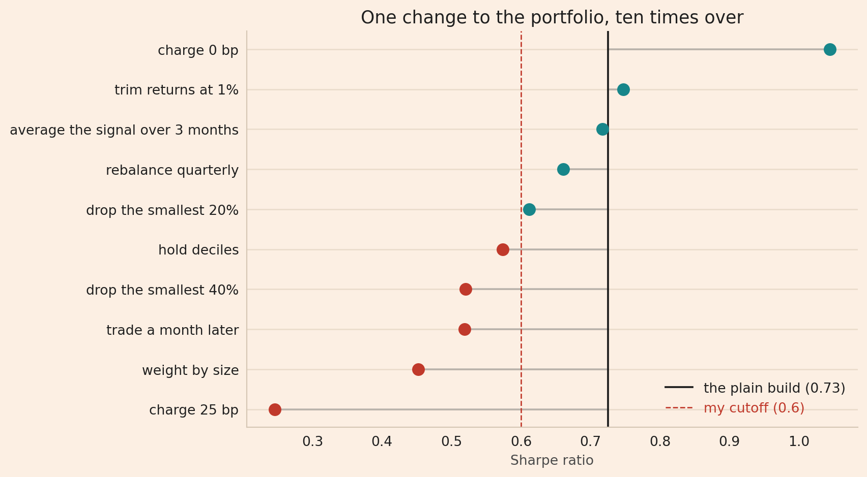
Each grey line starts at the plain build, the dark vertical line, and ends where one change leaves the Sharpe ratio. A red dot marks a change that takes the Sharpe ratio below my cutoff, the dashed line, and five of the ten changes do. Charging 25 basis points instead of 10 takes the Sharpe ratio from 0.73 to 0.25. Weighting by size takes the Sharpe ratio to 0.45. Holding deciles, the top and bottom tenth of the stocks instead of fifths, increases the return to 3.36% and decreases the Sharpe ratio to 0.57. And each of these changes is one line of code.
Running every combination
The ten single changes leave the other seven choices at the plain build. Running every combination of the eight choices, two options for six of them and three for the other two, gives 2⁶ × 3² = 576 versions of the same portfolio. Simonsohn and co-authors (2020) call a report of all such versions, instead of one preferred build, a specification curve.
# itertools.product takes the list of alternatives for each choice and returns every way
# of picking one value from each list, which is 576 combinations for these eight choices.
COMBOS = list(itertools.product(*FORKS.values()))

results_per_build = []
for combination in COMBOS:
    # zip pairs each choice name with its value in this combination, and dict turns those
    # pairs into the named arguments build expects.
    settings = dict(zip(KEYS, combination))
    monthly_pnl = build(panel_size, panel_signal, panel_return, **settings)
    results_per_build.append(report(monthly_pnl))

all_results = np.array(results_per_build)

# report hands back the annual return first and the Sharpe ratio second, so those are the
# two columns of all_results, one row per build.
annual_returns = all_results[:, 0]
sharpe_ratios = all_results[:, 1]

print(f"{len(COMBOS)} builds: {annual_returns.min():+.2f}%"
      f" to {annual_returns.max():+.2f}% a year,"
      f" Sharpe {sharpe_ratios.min():.2f} to {sharpe_ratios.max():.2f}")
for sharpe_cutoff in (0.5, 0.6, 0.7):
    builds_above = (sharpe_ratios > sharpe_cutoff).sum()
    print(f"  above a Sharpe of {sharpe_cutoff}: {builds_above} of {len(sharpe_ratios)}")
576 builds: -1.60% to +6.31% a year, Sharpe -0.17 to 1.07
above a Sharpe of 0.5: 211 of 576
above a Sharpe of 0.6: 126 of 576
above a Sharpe of 0.7: 70 of 576The reported return spans -1.60% to +6.31% a year, and the Sharpe ratio -0.17 to 1.07, on one dataset with one edge. At the cutoff of 0.6, I would trade 126 of the 576 builds. As a check on the cutoff: at 0.5, 211 of the 576 builds are above it, and at 0.7, 70 are.
Repeating the changes on one hundred datasets
One dataset is one draw, so, as a robustness check, I repeat the ten single changes on 100 fresh datasets, each built with the same edge.
# The ten single changes again, this time as (choice, alternative) pairs to loop over.
SINGLES = []
for choice in KEYS:
    for alternative in FORKS[choice]:
        if alternative != BASE[choice]:
            SINGLES.append((choice, alternative))

flips_per_dataset = []
for dataset_number in range(100):
    fresh_size, fresh_signal, fresh_return = make_panel(4000 + dataset_number)

    fresh_plain_pnl = build(fresh_size, fresh_signal, fresh_return, **BASE)
    # Unpacking both numbers names them, and only the Sharpe ratio is used from here.
    fresh_plain_return, fresh_plain_sharpe = report(fresh_plain_pnl)
    plain_passes = fresh_plain_sharpe > CUTOFF

    crossings = 0
    for single_choice, single_alternative in SINGLES:
        settings = {**BASE, single_choice: single_alternative}
        single_pnl = build(fresh_size, fresh_signal, fresh_return, **settings)
        single_return, single_sharpe = report(single_pnl)
        # A crossing is a change that puts the build on the other side of the cutoff from
        # where the plain build is, in either direction.
        if (single_sharpe > CUTOFF) != plain_passes:
            crossings += 1
    flips_per_dataset.append(crossings)

flips = np.array(flips_per_dataset)
print(f"at least one single change crosses the cutoff: {(flips > 0).mean():.0%} of datasets")
print(f"median number that do: {np.median(flips):.0f} of {len(SINGLES)}")
at least one single change crosses the cutoff: 79% of datasets
median number that do: 2 of 10On the dataset used up to here, five of the ten changes crossed my cutoff. Across the 100 datasets, the median number of changes that cross the cutoff, the middle value when the 100 counts are sorted, is two, and in 79% of the datasets at least one change moves the Sharpe ratio across the cutoff. So, which change flips the conclusion depends on the dataset, and in most datasets at least one change does.
Limitations
Eight choices are not 164 teams. Menkveld’s teams disagreed about what the hypothesis meant, which test to run, and how often to sample the data, and one team reported a trend of +74,491%. My eight choices copy none of that. I also do not know how often each of these choices is made in practice. So, the test shows the mechanism, and it does not measure how much real quants disagree.
Some builds are different strategies. A size-weighted decile portfolio can be called a different strategy from an equal-weighted quintile one. Part of the variation comes from disagreement about how to build one portfolio, and part comes from comparing two different portfolios.
The costs are assumptions too. I charge one flat rate on turnover. Novy-Marx and Velikov (2016) show that realistic costs vary across strategies and across stocks, so the 10 and 25 basis points are assumptions, like every other number in the build.
Turnover is simplified. Between scheduled rebalances the code keeps the target weights fixed, both for the return and for turnover, and ignores how price moves change the actual weights. So, between rebalances each build earns returns as if it were reset to its targets every month without cost. Tracking the actual weights would change the results.
The size of the edge is an assumption. I set the edge so that the plain build’s Sharpe ratio, 0.73, is above the cutoff of 0.6. I do not vary the size of the edge, so these counts apply to the edge I set.
Conclusion
The edge was in the data the whole time. How I built the portfolio decided the conclusion, and every choice in the build was ordinary.
For a backtest, the nonstandard error is the spread of results that ordinary build choices produce from one dataset. A single Sharpe ratio is one build out of the 576 here. Charging 25 basis points instead of 10 takes the Sharpe ratio from 0.73 to 0.25, from one side of my cutoff to the other, without an error in either build.
So, report the choices next to the result. Give the turnover and the cost you charged. Show the result with and without the stocks you dropped. And when the Sharpe ratio is near the cutoff, say which choices would put the Sharpe ratio on the other side of the cutoff, because another quant may make some of those choices differently.
The takeaway is that a backtest reports one build of the strategy, so before trading the strategy, ask how many of the other reasonable builds agree.
Read next
- Trading costs more than halved Swedish momentum’s ending value What trading costs did to a momentum portfolio on Swedish stocks.
- Does your backtested Sharpe ratio show a real edge? The other problem with one number: too few observations behind it.
Disclaimer: a simplified, hypothetical backtest on simulated data, for discussion purposes only. I put the edge into the data myself. Not investment advice. Past performance does not guarantee future returns.
Sources: Albert Menkveld and co-authors, Nonstandard Errors, Journal of Finance (2024). Amar Soebhag, Bart van Vliet and Patrick Verwijmeren, Non-standard errors in asset pricing: Mind your sorts, Journal of Empirical Finance (2024). Robert Novy-Marx and Mihail Velikov, A Taxonomy of Anomalies and Their Trading Costs, Review of Financial Studies (2016). Uri Simonsohn, Joseph Simmons and Leif Nelson, Specification curve analysis, Nature Human Behaviour (2020).