6,020 daily log returns, mean -0.00013, daily standard deviation 0.0100Purged cross-validation: why a model with no predictive power can score 90% accuracy
Python
Machine Learning
Backtesting
Tutorial
Code
Training labels that reach into the test period raise a model’s accuracy on returns with no signal to 90.5%, and dropping those training days gives 50.3%.
A model that predicts each day by copying the outcome of the most recent training day scores 90.5% accuracy, the share of correct predictions, on returns that contain no signal, although every training day comes before the day it predicts. The same model scores 50.3% once I drop the training days whose outcomes overlap the test day.
Say the outcome is the cumulative return over the next 20 days. We have 200 days of data and split them in half. The training set, which the model learns from, is days 1 to 100, and the test set, on which the model is scored, is days 101 to 200. The outcome for training day 100 is the return over days 101 to 120, and those days are in the test set. Every training day from 81 onward has an outcome that extends beyond day 100 into the test period, so those training outcomes already include test-period returns.
The fix is to purge: drop the training days near the boundary whose outcomes overlap the test period. The picture below shows the split before and after purging.
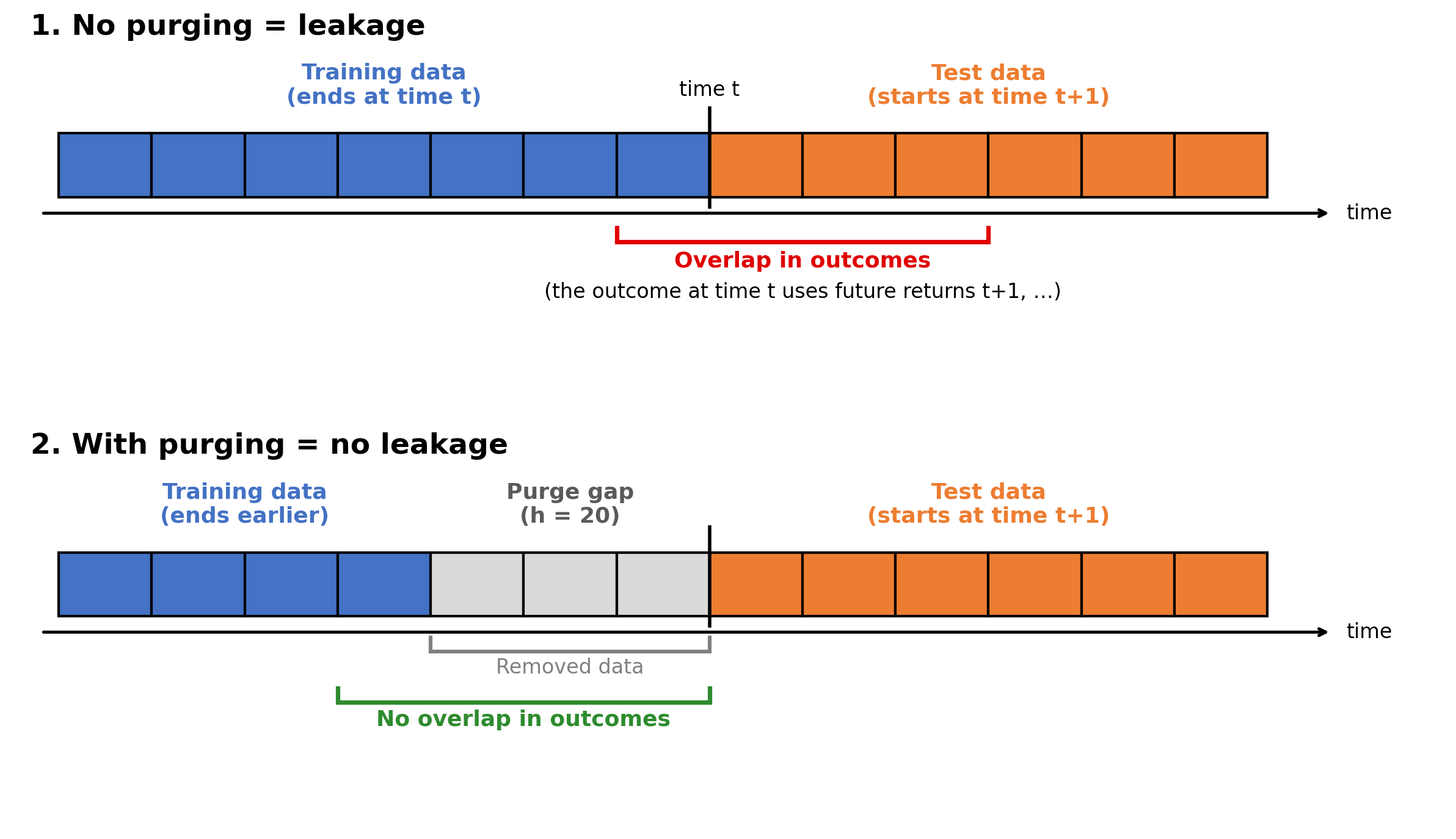
A training outcome that overlaps the test period is a form of look-ahead bias: the model learns from returns of the test period.
Step 1. Simulating the data
I simulate the returns myself, so I know the truth up front: there is nothing to predict. Each day’s return is
\[r_t = 0.01\,z_t,\]
where \(z_t\) is a draw from the standard normal distribution, which is bell-shaped with a mean of 0 and a standard deviation of 1, the standard deviation being a measure of how far values typically are from their mean. So each day’s return has a mean of zero and a standard deviation of 1%, independently of every other day.
NoteCode: the returns
import numpy as np                  # arrays and math
import pandas as pd                 # tables and dates

HORIZON = 20                        # the outcome looks 20 trading days ahead
N = 6_000                           # how many days we will label

# A fixed seed makes the generator hand back the same draw on every run, so the numbers
# printed on this page are the numbers you get when you run the code yourself.
random_generator = np.random.default_rng(7)

# We need N days to label, plus HORIZON extra days so the last label still has
# a full 20-day future to look at. That is N + HORIZON returns in total.
total_days = N + HORIZON

dates = pd.bdate_range("2000-01-03", periods=total_days)      # business days only
daily_moves = random_generator.normal(0, 0.01, total_days)    # mean 0, 1% daily standard deviation
ret = pd.Series(daily_moves, index=dates)                     # one log return per date

print(f"{len(ret):,} daily log returns, mean {ret.mean():+.5f}, daily standard deviation {ret.std():.4f}")The block prints 6,020 simulated daily returns, 20 more than the 6,000 days that get a label, because the last label needs the 20 returns after it. Their mean is −0.013% a day and their standard deviation 1.00%, as the formula sets.
Step 2. Defining the outcome: up or down over the next 20 days
The model predicts whether the return over the next 20 trading days is positive or negative. The daily returns are log returns, \(r_t = \ln(P_t/P_{t-1})\), the logarithm of the day’s price ratio, and log returns add up over days, so the sum of the next 20 is exactly the 20-day log return. Day \(t\) is labelled 1 if that sum is positive and 0 if it is not:
\[y_t = \begin{cases} 1 & \text{if } r_{t+1} + r_{t+2} + \dots + r_{t+20} > 0, \\ 0 & \text{otherwise.} \end{cases}\]
NoteCode: the labels
# rolling(HORIZON) walks a 20-day window along the series, and sum() adds each window up.
# The total is on the LAST day of the window it came from.
rolling_20_day_sum = ret.rolling(HORIZON).sum()

# shift(-HORIZON) moves every value 20 rows earlier, so each total is on the day
# just BEFORE its own window. Every day then has the return of its own next 20 days.
future = rolling_20_day_sum.shift(-HORIZON)

# The last HORIZON days have no complete future left, so only the first N days get a label.
future_of_labelled_days = future.iloc[:N]
rose_over_next_20_days = future_of_labelled_days > 0    # a Series of True and False
y = rose_over_next_20_days.astype(int).to_numpy()       # True becomes 1, False becomes 0

print(f"{len(y):,} labels, {y.mean():.1%} of them positive")
6,000 labels, 48.4% of them positiveAbout 48% of the labels are positive, close to the 50% expected from returns that are as likely to be positive as negative. Since future returns are independent of all past information by construction, a valid test should produce accuracy around 50%. The 90.5% accuracy of step 4 therefore cannot come from predictive skill.
Step 3. Measuring how much neighboring labels overlap
The issue is in how the outcome is built: each day’s label uses the 20 returns that follow it, so two neighboring labels share 19 of their 20 returns. The block below lines up two neighboring days.
NoteCode: two neighboring labels
day = 100                # any day would do, and this one is only an example
next_day = day + 1       # the day immediately after day 100

print(f"day {day}'s label uses returns {next_day} to {day + HORIZON}")
print(f"day {next_day}'s label uses returns {next_day + 1} to {next_day + HORIZON}")
print(f"the two overlap on returns {next_day + 1} to {day + HORIZON}: {HORIZON - 1} of {HORIZON}")
day 100's label uses returns 101 to 120
day 101's label uses returns 102 to 121
the two overlap on returns 102 to 120: 19 of 20Moving the window forward one day drops its first return and adds one new return. The other 19 returns stay the same, so the two totals often have the same sign. The block below counts how often neighboring labels agree across the whole series.
NoteCode: how often neighboring labels agree
# y[:-1] is every label except the last one, and y[1:] is every label except the first.
# Lining the two arrays up puts each label beside the label of the day after it.
label_today = y[:-1]
label_next_day = y[1:]
labels_match = label_today == label_next_day   # one True or False per pair of days

agree = labels_match.mean()                    # the mean of True and False is the share of True
print(f"neighboring labels agree {agree:.0%} of the time")
neighboring labels agree 91% of the timeSo, neighboring labels agree about 91% of the time, and the overlapping returns raise the agreement above the 50% expected from independent labels. The copying model of the next step is right whenever neighboring labels agree.
Step 4. Running the naive test
To test a model, I use walk-forward validation. Instead of a single 50:50 split, I test one day at a time, always training only on earlier days and then rolling forward. The last 3,600 of the 6,000 labelled days are the test days, and each is predicted by a model trained on the 252 days before it, about a trading year. Since every training day comes before its test day, the test appears to use no future information.
The model’s only input, its feature, is the day’s number, 0, 1, 2, ..., which contains no information about future returns. The model is a one-nearest-neighbor classifier, which means that to label a test day, it finds the single closest training day and copies that day’s label. Since the feature is the day number, the closest training day is always the last training day before the test day.
NoteCode: the naive test
from sklearn.model_selection import TimeSeriesSplit     # rolling splits, past before future
from sklearn.neighbors import KNeighborsClassifier      # the "copy the closest past day" model
from sklearn.metrics import accuracy_score              # share of predictions that were correct

# sklearn wants a table with one row per observation and one column per feature, even when
# there is a single feature. reshape(-1, 1) turns the day numbers into a single column,
# and the -1 tells numpy to work out how many rows that takes.
day_numbers = np.arange(N)
X = day_numbers.reshape(-1, 1)                          # the feature: day 0, 1, 2, ...


def walk_forward(gap):
    """Test one day at a time and return the share of test days the model got right.

    gap is how many days are dropped between the end of the training block and the test day.
    """
    # 3600 splits, so 3600 test days. test_size=1 makes each test set a single day, and
    # max_train_size=252 caps the training block at 252 days, about a trading year.
    splitter = TimeSeriesSplit(n_splits=3_600, test_size=1, max_train_size=252, gap=gap)

    true_labels = []
    predictions = []

    # split() hands back the row positions of the training days and of the test day.
    for train_rows, test_rows in splitter.split(X):
        model = KNeighborsClassifier(n_neighbors=1)     # 1 neighbor: copy the closest day
        model.fit(X[train_rows], y[train_rows])         # "learn" from the training days
        predicted_labels = model.predict(X[test_rows])  # an array holding one label
        predictions.append(predicted_labels[0])
        true_labels.append(y[test_rows][0])         # the answer we are trying to match

    return accuracy_score(true_labels, predictions)


naive = walk_forward(gap=0)                             # no gap between training and test
print(f"walk-forward, no gap:   {naive:.1%}")
walk-forward, no gap: 90.5%The model scores 90.5%, even though the feature predicts nothing and the returns contain no signal. A score that high on data with no edge means that information about the test days has leaked into training.
Step 5. Looking at what the model copied
To see where the leak comes from, I open up the very first split and look at which training day the model copied.
NoteCode: the first split
def first_split(gap):
    """Report on the very first train/test split that walk_forward would use.

    It gives back the last training day, the test day, how many days apart the two are,
    and how many of their twenty returns the two labels share.
    """
    splitter = TimeSeriesSplit(n_splits=3_600, test_size=1, max_train_size=252, gap=gap)

    # split() produces one pair of row positions per split, and next() takes the first pair
    # and then stops, so nothing after the first split is built.
    train_rows, test_rows = next(splitter.split(X))

    last_training_day = train_rows[-1]                  # the newest day the model trained on
    test_day = test_rows[0]                             # the day it has to predict
    days_apart = test_day - last_training_day

    # Labels one day apart share 19 of their 20 returns, two days apart 18, and so on.
    # Once they are HORIZON days apart they share none, and max() holds the count at zero
    # instead of letting it go negative.
    shared_returns = max(HORIZON - days_apart, 0)

    return last_training_day, test_day, days_apart, shared_returns


# Unpacking gives each returned value its own name, in the order the function lists them.
last_training_day, test_day, days_apart, shared_returns = first_split(gap=0)
print(f"last training day: {last_training_day}")
print(f"test day:          {test_day}")
print(f"days apart:        {days_apart}")
print(f"returns their labels share: {shared_returns} of {HORIZON}")
last training day: 2399
test day: 2400
days apart: 1
returns their labels share: 19 of 20The most recent training day is one day before the test day, and their labels share 19 of their 20 returns, so copying the neighboring day’s label is right as often as neighboring labels agree. Step 3 measures that agreement at 91% across all 6,000 labels, and the walk-forward test measures 90.5% accuracy across the 3,600 test days.
Step 6. Purging the overlap
The fix follows from the diagnosis: drop the training days whose outcomes are not complete before the test day. In scikit-learn’s TimeSeriesSplit, that takes one argument, gap. With gap=20, the 20 days before the test day are left out of training, so for test day 100 the latest training day is 79, whose outcome uses the returns of days 80 to 99. Every training outcome then ends before the test day, so no training label shares a return with the test label. A gap of 20 days, the full horizon, is enough, and here a gap of 19 would also leave no shared returns.
NoteCode: the purged test
# The same inspection as in Step 5, with the gap in place this time.
last_training_day, test_day, days_apart, shared_returns = first_split(gap=HORIZON)
print(f"last training day {last_training_day}, test day {test_day}, "
      f"{days_apart} days apart, labels share {shared_returns} returns")

purged = walk_forward(gap=HORIZON)                        # the only change is the gap
print(f"walk-forward, {HORIZON}-day gap: {purged:.1%}")
last training day 2379, test day 2400, 21 days apart, labels share 0 returns
walk-forward, 20-day gap: 50.3%With the gap in place, the nearest training label is now 21 days before the test label and shares none of the test label’s returns. Accuracy is 50.3%, close to the 50% expected when the returns contain no signal. The only change between the two tests is the gap, so the whole difference between 90.5% and 50.3% comes from training labels whose returns overlapped the test label’s returns.
The simpler form of the same error, a signal acted on before it was available, is Lesson 30 in Practical Coding.
Step 7. Comparing the results
Finally, the chart below puts the three numbers side by side: the naive test, the purged test, and the 50% we would expect from chance alone.
NoteCode: the chart
import matplotlib.pyplot as plt

RED, TEAL, ORANGE, GREY = "#C0392B", "#17868A", "#D2822B", "#888888"
# The site's chart colours: a cream background, a light grid and a pale frame, so every chart
# on the site has the same look.
BG, INK, GRID, SPINE, AXIS_TEXT = "#FCEFE3", "#1f1f1f", "#EADCCC", "#D5C6B4", "#4a4a4a"


def style_chart(figure, axis):
    """Give a finished chart the site's cream background, light grid and pale frame."""
    figure.patch.set_facecolor(BG)
    axis.set_facecolor(BG)
    axis.grid(True, axis="y", color=GRID, lw=1.0)
    axis.set_axisbelow(True)
    for side in ("top", "right"):
        axis.spines[side].set_visible(False)
    for side in ("left", "bottom"):
        axis.spines[side].set_color(SPINE)
    axis.tick_params(axis="both", length=0, colors=INK, pad=6)
    axis.xaxis.label.set_color(AXIS_TEXT)
    axis.yaxis.label.set_color(AXIS_TEXT)
    axis.title.set_color(INK)
    # Each legend entry in the colour of what it labels: a line's colour or a bar's fill.
    # get_legend() returns None when the chart has no legend.
    legend = axis.get_legend()
    if legend is not None:
        for text, handle in zip(legend.get_texts(), legend.legend_handles):
            if hasattr(handle, "get_color"):
                text.set_color(handle.get_color())
            else:
                text.set_color(handle.get_facecolor())


# The returns are symmetric around zero, so pure chance is 50%. That is the chance benchmark.
bar_labels = ["naive\n(no gap)", f"purged\n({HORIZON}-day gap)", "chance\n(50%)"]
bar_heights = [naive * 100, purged * 100, 50.0]

plt.figure(figsize=(7, 4.5))
bars = plt.bar(bar_labels, bar_heights, color=[RED, TEAL, GREY])
plt.ylim(0, 100)                                          # full axis, so the difference between the bars is not exaggerated
plt.ylabel("accuracy (%)")
plt.title("Accuracy with no gap, with a 20-day gap, and by chance")
plt.bar_label(bars, fmt="%.1f%%", padding=3, color=INK)   # print each value on top of its bar
style_chart(plt.gcf(), plt.gca())       # gcf and gca are the current figure and axis
plt.tight_layout()
plt.savefig("purging_accuracy.png", dpi=120, bbox_inches="tight", facecolor=BG)
plt.show()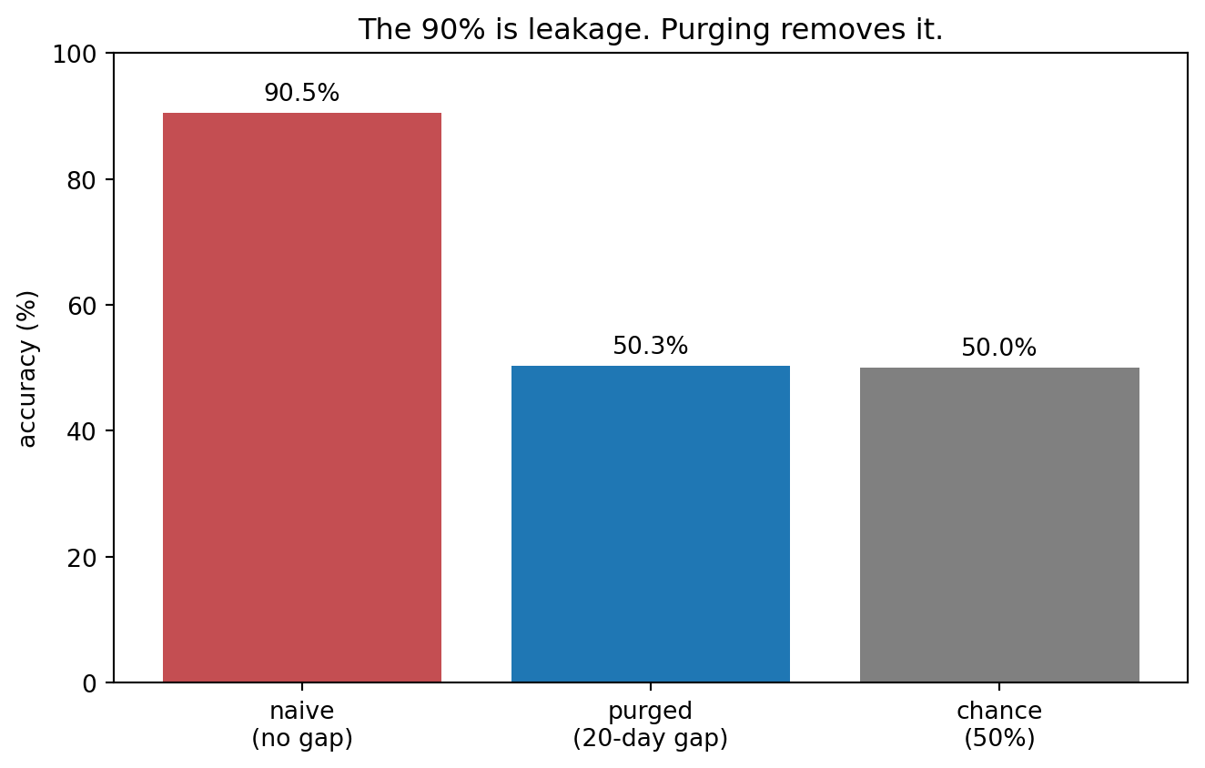
The red bar is the naive test, the teal bar the purged test, and the grey bar chance. Ignoring the label overlap inflates measured accuracy by 40.2 percentage points in this example, from 50.3% to 90.5%.
Limitations
Accuracy is not profit. Getting the direction right tells us nothing about the size of the gains and losses, or about trading costs, so a strategy can be accurate and still lose money.
The example is extreme on purpose. The day-number feature and the copy-the-neighbor model make the leak unusually large and easy to see. The underlying problem is general: whenever a training label overlaps the test period, that training row already contains part of the test label’s returns. How much a given model exploits the overlap depends on the labels, the features, the model and the validation design.
Purging only fixes this particular leakage. Purging removes the overlap between training and test outcomes, but other kinds of leakage remain, such as features built from forward-looking windows, or features rescaled with a mean and standard deviation computed from the whole sample, test days included.
Conclusion
Ordering the data in time is only the first step. The takeaway is that when the outcome spans several future days, every training outcome has to end before the test period starts. Otherwise, as here, a model with no information about future returns scores 90.5% instead of 50.3%.
Read next
- In a market with no edge, tuning against the hold-out produced a Sharpe ratio of 2.8 How a hold-out gets used up once we start tuning against it.
- Does your backtested Sharpe ratio show a real edge? Separating a real edge from luck with a bootstrap.
Disclaimer: a teaching example on simulated data. The returns are generated and contain no signal by construction. Not investment advice.
Sources: Marcos López de Prado, Advances in Financial Machine Learning (2018), ch. 7 on cross-validation in finance. Stefan Jansen, Machine Learning for Algorithmic Trading, 2nd ed. (2020), ch. 6 on purging and embargoing. scikit-learn, TimeSeriesSplit.