import numpy as np

rng = np.random.default_rng(0)
N, HOLDOUT, FINAL = 30, 756, 2520          # 30 assets; 3-year hold-out; 10-year final test

# Independent zero-mean daily returns. Nothing predicts anything.
Rh = rng.normal(0, 0.01, (HOLDOUT, N))     # the hold-out I will keep checking
Rt = rng.normal(0, 0.01, (FINAL,   N))     # the final test, opened once at the end

def sharpe(x):
    x = np.asarray(x)
return x.mean() / x.std(ddof=1) * np.sqrt(252) # annualised Sharpe ratioWhen out of sample stops being out of sample
Python
Backtesting
Statistics
Code
On a simulated market with no edge, a researcher who keeps tuning against a hold-out drives its Sharpe ratio to 2.8, while a final test set opened once stays at zero. Your out-of-sample test becomes in-sample the moment you optimise against it.
You split your history in two. You build the strategy on the first part and keep the second part untouched, according to the textbook. Although that sounds right, research is rarely one-and-done.
Say you test the strategy on the hold-out and it disappoints. So, you lengthen the lookback and run it again. Still weak, so you add a volatility filter and run it again. Then you drop the smallest names and run it again. You might have several ideas you want to test, to see which one works. The issue is that the supposed out-of-sample starts becoming in-sample, because you are changing the strategy after seeing its out-of-sample results. Data that was meant to be new and unseen becomes data you have already looked at.
In this post I show how far this can go. I build a market where nothing can be predicted, so an honest test of any strategy should land near a Sharpe ratio of zero. I then set aside two test sets from that market: a hold-out that I check after every change, and a final test that I do not open until the strategy is finished. After 1,500 rounds of tuning, the hold-out shows a Sharpe ratio of 2.8, which looks like a strong strategy. The final test shows roughly zero, which is the truth. Dwork and co-authors (2015) call this adaptive data analysis: a hold-out stops being independent the moment its results start guiding your choices.
Step 1. A market with no edge
I simulate the market myself, so I know the truth up front: there is nothing to find. Each day, every one of the thirty assets gets a return drawn independently from a bell curve centred on zero, so yesterday’s return says nothing about today’s. I then split this market in two: three years become the hold-out, and ten years become the final test.
Step 2. Tune against the hold-out
The strategy is a portfolio of the thirty assets. Then in each round I change one weight by a small random amount and test the new version on the hold-out. If the hold-out Sharpe ratio improves, I keep the change, and if it worsens, I go back to the previous version. Each change is one small research idea, like the longer lookback or the volatility filter from the introduction, and I try 1,500 of them.
w = np.zeros(N); w[rng.integers(N)] = 1.0        # start from one asset
best_h = sharpe(Rh @ w)
holdout_path, test_path = [], []

for _ in range(1500):                            # 1500 rounds of check and tweak
    j = rng.integers(N)
    w_try = w.copy(); w_try[j] += rng.normal(0, 0.25)   # change one weight a little
    h = sharpe(Rh @ w_try)
    if h > best_h:                               # keep the change only if the hold-out improved
        w, best_h = w_try, h
    holdout_path.append(best_h)                  # the hold-out Sharpe I would be reporting
    test_path.append(sharpe(Rt @ w))             # what the final test would say right now
I record two numbers each round: the Sharpe ratio on the hold-out, which I see and react to, and the Sharpe ratio the same strategy would have on the final test, which stays hidden until the end.
Step 3. What the two sets say
print(f"kept changes:      {int(np.sum(np.diff(holdout_path) > 0))} of 1500")
print(f"hold-out Sharpe:   {holdout_path[-1]:+.2f}")
print(f"final test Sharpe: {test_path[-1]:+.2f}")
kept changes: 244 of 1500
hold-out Sharpe: +2.78
final test Sharpe: -0.21Out of the 1,500 tries, about 240 changes made the hold-out better and stayed. Together they took the hold-out Sharpe ratio from below zero to 2.8. The same strategy, scored once on the final test, comes out at minus 0.2. It looks like a good strategy. But this market contains nothing to predict, so the 2.8 comes entirely from checking the same three years 1,500 times.
Results
import matplotlib.pyplot as plt

fig, ax = plt.subplots(figsize=(9, 4.6))
ax.plot(holdout_path, color="#C44E52", lw=1.9, label="hold-out (tuned against)")
ax.plot(test_path,    color="#1F77B4", lw=1.9, label="final test (opened once)")
ax.axhline(0, color="#888", lw=0.9)
ax.set_xlabel("number of hold-out checks"); ax.set_ylabel("Sharpe ratio")
ax.set_title("Tuning against the hold-out inflates only the hold-out")
ax.legend(frameon=False)
plt.tight_layout(); plt.savefig("oos_overfitting.png", dpi=140, bbox_inches="tight"); plt.show()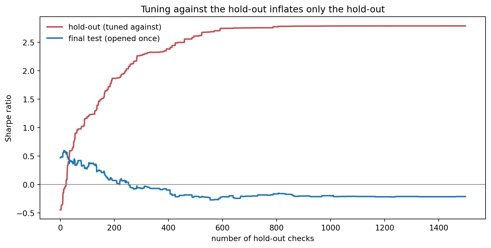
The red line is the hold-out, and it rises in small steps as I keep more changes. The blue line is the final test for the very same strategy, and it stays around zero the whole way.
The rise has a plain cause. In any three years of noise, a few assets end up with a positive average return by luck alone. A change that puts more weight on one of them makes the hold-out Sharpe ratio better, so I keep it, and round after round the strategy ends up holding the assets that were lucky in the hold-out. The final test has its own lucky assets, and they are different ones, so the same strategy earns nothing there.
Where the line is
A hold-out stays out of sample only while its results do not change what you do next. Check it once, against a rule you set in advance, and it keeps its meaning. Check it, adjust, and check again, and each adjustment fits the strategy a little more to that particular sample. After enough rounds, the hold-out score mostly measures how long you searched.
What this does not settle
This is not the same as testing many strategies at once. The best of many strategies looks strong by chance alone, which I cover in an earlier post. Here there is one strategy, changed step by step after each look at the hold-out.
Real research leaks more than this. My loop only changes weights, while a real project also picks which years to include, which names to drop, and when to stop, each after seeing the last result. Every one of those choices is another check.
Simulated data shows the mechanism, and it cannot show the size. How badly a real hold-out inflates depends on the data, on how freely you search, and on how many times you check.
What it means
Decide in advance what result counts as a pass. Then run the finished strategy on the final test once, and let the result stand. If it fails and you go back to research, those years are used up, and the next version of the strategy needs a test that is still untouched. The cleanest such test is data that did not exist while you were working, which is why a finished strategy is usually paper-traded, run forward on new days without real money, before any money follows it. The takeaway is that a hold-out stops being out of sample the moment you optimise against it, because the person doing the optimising is part of what gets fitted.
Read next
- Does your backtested Sharpe ratio show a real edge? The companion problem: picking the best of many strategies at once, and how a bootstrap exposes it.
- Why a model with no predictive power can score 90% accuracy Another way validation lies, this time through outcomes that overlap in time.
Disclaimer: a teaching example on simulated data. The returns are generated and contain no edge by construction. Not investment advice.
Sources: Dwork, Feldman, Hardt, Pitassi, Reingold and Roth, “The reusable holdout: preserving validity in adaptive data analysis” (Science, 2015). For the finance framing, Bailey and López de Prado (2014) on the deflated Sharpe ratio and backtest overfitting, and Harvey and Liu (2015), “Backtesting”, on multiple testing.