Two models with 99% accuracy can rank an offender differently

How accuracy and the AUC differ, shown with two models that both have 99% accuracy on 100 traders but AUCs of 0.50 and 0.91.

Source: Image by author using ChatGPT

Say we have 100 traders and, in truth, one of them, the offender, committed a market crime. A model gives every trader a score between 0 and 1, higher for a trader who looks more suspicious, and flags every trader whose score is at least a threshold, here 0.5. A constant model gives every trader the same low score and so flags no trader. It uses no information about the traders and is still right about all 99 non-offenders, so its accuracy, the share of correct predictions, is 99%.

So, the issue is that accuracy counts every correct prediction equally, and when offenders are rare, almost every correct prediction is for a non-offender. A surveillance model can give the offender a higher score than 90 of the 99 non-offenders and still flag no trader, if every score is below the threshold. Its accuracy is then also 99%, so accuracy cannot show that it ranks the offender above most non-offenders.

In this post I use the scores of the two models to build the receiver operating characteristic (ROC) curve and the area under it (AUC). The AUC is the share of correctly ordered pairs: pairs of one offender and one non-offender in which the offender has the higher score, counting a tie as half. The constant model has an AUC of 0.50, the same as ordering each pair with a coin flip, and the surveillance model has an AUC of 0.91.

Comparing two models with the same accuracy

I build the traders myself, so I know which one is the offender. Each trader has a label, 1 for the offender and 0 for a non-offender, and each model gives a prediction, 1 when it flags the trader and 0 otherwise. The block below builds the constant model, which gives every trader a score of 0.01, and counts its correct predictions.

import numpy as np

NUMBER_OF_TRADERS = 100
THRESHOLD = 0.5          # a trader with a score of 0.5 or higher is flagged

# One label per trader: 1 for the offender and 0 for a non-offender.
# np.zeros builds an array of 100 zeros. dtype=int stores them as 0 instead of 0.0.
is_offender = np.zeros(NUMBER_OF_TRADERS, dtype=int)
is_offender[0] = 1                                   # position 0 is the offender

# np.full builds an array of 100 scores, all equal to 0.01.
constant_scores = np.full(NUMBER_OF_TRADERS, 0.01)

# constant_scores >= THRESHOLD is True for a trader with a score of 0.5 or higher and
# False otherwise. astype(int) turns True into 1 and False into 0, like the labels.
constant_predictions = (constant_scores >= THRESHOLD).astype(int)

# Adding up the predictions counts the 1s, which is the number of flagged traders.
# constant_predictions == is_offender is True where a prediction equals the label, and
# np.sum counts each True as 1, which gives the number of correct predictions.
traders_flagged = np.sum(constant_predictions)
correct_predictions = np.sum(constant_predictions == is_offender)
constant_accuracy = correct_predictions / NUMBER_OF_TRADERS

# In an f-string, :.0% prints a number as a percentage with no decimals: 0.99 as 99%.
print(f"traders flagged:     {traders_flagged} of {NUMBER_OF_TRADERS}")
print(f"correct predictions: {correct_predictions} of {NUMBER_OF_TRADERS}")
print(f"accuracy:            {constant_accuracy:.0%}")

traders flagged:     0 of 100
correct predictions: 99 of 100
accuracy:            99%

The surveillance model gives higher scores to traders whose trading looks more suspicious. I set its scores so that every number can be checked by hand: the offender scores 0.40, nine non-offenders score 0.45, and the other 90 score 0.10. The block below shows one trader with each score for both models, where position is the trader’s row in the data and row 0 is the offender, and checks whether the two models make the same predictions.

import pandas as pd

# Give all 100 traders a score of 0.10, then change the scores of ten traders.
surveillance_scores = np.full(NUMBER_OF_TRADERS, 0.10)
surveillance_scores[0] = 0.40          # position 0, the offender
surveillance_scores[1:10] = 0.45       # [1:10] is positions 1 to 9, nine non-offenders

surveillance_predictions = (surveillance_scores >= THRESHOLD).astype(int)
surveillance_accuracy = np.mean(surveillance_predictions == is_offender)

# One trader with each score: position 0 is the offender, position 1 scores 0.45,
# and position 10 scores 0.10.
example_positions = [0, 1, 10]
example_traders = pd.DataFrame({
    "position": example_positions,
    "label": is_offender[example_positions],
    "constant score": constant_scores[example_positions],
    "constant prediction": constant_predictions[example_positions],
    "surveillance score": surveillance_scores[example_positions],
    "surveillance prediction": surveillance_predictions[example_positions],
})

# index=False leaves out the row numbers. float_format="{:.2f}".format prints every
# decimal number with two decimals, such as 0.40.
print(example_traders.to_string(index=False, float_format="{:.2f}".format))

# np.array_equal is True only when the two arrays match at every position.
same_predictions = np.array_equal(constant_predictions, surveillance_predictions)
print(f"\nsame predictions for all {NUMBER_OF_TRADERS} traders: {same_predictions}")
print(f"accuracy of the surveillance model:   {surveillance_accuracy:.0%}")

 position  label  constant score  constant prediction  surveillance score  surveillance prediction
        0      1            0.01                    0                0.40                        0
        1      0            0.01                    0                0.45                        0
       10      0            0.01                    0                0.10                        0

same predictions for all 100 traders: True
accuracy of the surveillance model:   99%

Every score of the surveillance model is below 0.5, so both models predict 0 for all 100 traders and both have an accuracy of 99%. Only the scores differ, so comparing how the two models rank the offender needs the scores.

Lowering the threshold

One way to use the scores is to lower the threshold. The surveillance model then flags the traders with the highest scores first, and it flags additional traders only when the threshold decreases to another score. A flagged offender is a true positive: the prediction is positive, 1, and correct. A flagged non-offender is a false positive: the prediction is positive and wrong. At each threshold, the block below calculates accuracy and three shares:

• True positive rate, also called recall: the share of offenders who are flagged.
• False positive rate: the share of non-offenders who are flagged.
• Precision: the share of flagged traders who are offenders.

def evaluate_threshold(labels, scores, threshold):
    """Flag every trader whose score is at least the threshold, and count the results.

    With labels [1, 0, 0], scores [0.40, 0.45, 0.10] and threshold 0.40, the first two
    traders are flagged: one offender and one non-offender, so precision is 0.5.
    """
    predictions = (scores >= threshold).astype(int)

    # & means "and" between two True/False arrays. (predictions == 1) & (labels == 1)
    # is True for a trader who is flagged and is an offender.
    offenders_flagged = np.sum((predictions == 1) & (labels == 1))
    non_offenders_flagged = np.sum((predictions == 1) & (labels == 0))
    traders_flagged = offenders_flagged + non_offenders_flagged

    # The true positive rate divides by the number of offenders, and the false positive
    # rate divides by the number of non-offenders.
    true_positive_rate = offenders_flagged / np.sum(labels == 1)
    false_positive_rate = non_offenders_flagged / np.sum(labels == 0)
    accuracy = np.mean(predictions == labels)

    # Precision divides by the number of traders flagged. When no trader is flagged, that
    # number is 0 and the division is undefined, so precision is set to np.nan, which
    # means "not a number" and prints as NaN.
    if traders_flagged == 0:
        precision = np.nan
    else:
        precision = offenders_flagged / traders_flagged

    # Return the results as a dictionary. When a list of these dictionaries becomes a
    # DataFrame below, each key becomes a column name.
    return {
        "threshold": threshold,
        "offenders flagged": offenders_flagged,
        "non-offenders flagged": non_offenders_flagged,
        "true positive rate": true_positive_rate,
        "false positive rate": false_positive_rate,
        "accuracy": accuracy,
        "precision": precision,
    }


# 0.50 is the threshold used so far. 0.45, 0.40 and 0.10 are the three different scores
# in surveillance_scores, from highest to lowest.
threshold_rows = []
for threshold in [0.50, 0.45, 0.40, 0.10]:
    row = evaluate_threshold(is_offender, surveillance_scores, threshold)
    threshold_rows.append(row)

threshold_table = pd.DataFrame(threshold_rows)
print(threshold_table.to_string(index=False, float_format="{:.2f}".format))

# The constant model at the threshold of 0.40, to compare with the surveillance model.
constant_row = evaluate_threshold(is_offender, constant_scores, 0.40)
print(f"\nconstant model at 0.40: accuracy {constant_row['accuracy']:.2f}, "
      f"true positive rate {constant_row['true positive rate']:.2f}")

 threshold  offenders flagged  non-offenders flagged  true positive rate  false positive rate  accuracy  precision
      0.50                  0                      0                0.00                 0.00      0.99        NaN
      0.45                  0                      9                0.00                 0.09      0.90       0.00
      0.40                  1                      9                1.00                 0.09      0.91       0.10
      0.10                  1                     99                1.00                 1.00      0.01       0.01

constant model at 0.40: accuracy 0.99, true positive rate 0.00

At 0.50 no trader is flagged, so precision, a share of the flagged traders, is undefined and prints as NaN, not a number. At 0.45, the model flags the nine non-offenders who score 0.45: nine false positives and an accuracy of 90%. At 0.40, it also flags the offender, its one true positive, so accuracy is 91%, the true positive rate 1.00, the false positive rate 9/99 = 0.09, and precision 0.10, one offender among ten flagged traders. At 0.10, the lowest score, every trader is flagged, so both rates are 1, and accuracy and precision are 0.01.

At 0.40, the constant model still flags no trader and keeps an accuracy of 99%: one error, the missed offender, against the surveillance model’s nine false positives. Accuracy counts errors at one threshold. Which model ranks the offender above the non-offenders is a different question, which the ROC curve answers at every threshold.

Drawing the ROC curve

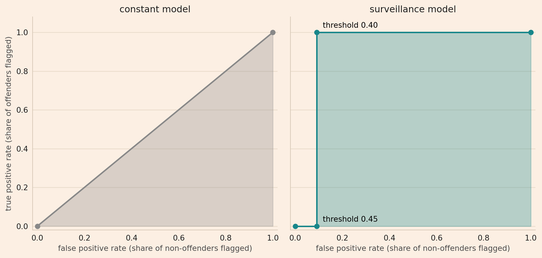
The ROC curve is a chart with one point per threshold: the false positive rate on the horizontal axis and the true positive rate on the vertical axis. Lowering the threshold moves along the curve from (0, 0), where no trader is flagged, to (1, 1), where every trader is flagged. A point higher up means more offenders flagged, and a point further right means more non-offenders flagged, so the top left corner is the point where every offender and no non-offender is flagged.

The curve shows how many non-offenders a model flags before it flags the offender. The block below computes the points of both curves, one per threshold, and the chart after it plots them, with the area under each curve shaded.

def roc_curve_points(labels, scores):
    """Return the false positive rate and true positive rate at each threshold.

    The first threshold is higher than every score, so no trader is flagged. The next
    thresholds are the different scores from highest to lowest, and at the lowest score
    every trader is flagged.
    """
    # np.unique lists each different score once, from lowest to highest. [::-1] reverses
    # that order, so highest_first runs from the highest score to the lowest.
    distinct_scores = np.unique(scores)
    highest_first = distinct_scores[::-1]

    # np.inf is infinity. Every score is below it, so at this first threshold no trader is
    # flagged. list() turns the numpy array into a Python list, because + joins two lists
    # into one longer list, while + with a numpy array adds numbers.
    thresholds = [np.inf] + list(highest_first)

    false_positive_rates = []
    true_positive_rates = []
    for threshold in thresholds:
        row = evaluate_threshold(labels, scores, threshold)
        false_positive_rates.append(row["false positive rate"])
        true_positive_rates.append(row["true positive rate"])
    return false_positive_rates, true_positive_rates


constant_false_positive_rates, constant_true_positive_rates = roc_curve_points(
    is_offender, constant_scores)
surveillance_false_positive_rates, surveillance_true_positive_rates = roc_curve_points(
    is_offender, surveillance_scores)

import matplotlib.pyplot as plt

GREY, TEAL = "#888888", "#17868A"
# The site's chart colours: a cream background, a light grid and a pale frame, so every chart
# on the site has the same look.
BG, INK, GRID, SPINE, AXIS_TEXT = "#FCEFE3", "#1f1f1f", "#EADCCC", "#D5C6B4", "#4a4a4a"


def style_chart(figure, axis):
    """Give a finished chart the site's cream background, light grid and pale frame."""
    figure.patch.set_facecolor(BG)
    axis.set_facecolor(BG)
    axis.grid(True, axis="y", color=GRID, lw=1.0)
    axis.set_axisbelow(True)
    for side in ("top", "right"):
        axis.spines[side].set_visible(False)
    for side in ("left", "bottom"):
        axis.spines[side].set_color(SPINE)
    axis.tick_params(axis="both", length=0, colors=INK, pad=6)
    axis.xaxis.label.set_color(AXIS_TEXT)
    axis.yaxis.label.set_color(AXIS_TEXT)
    axis.title.set_color(INK)
    # each legend entry in the colour of its line; get_legend() returns None without a legend
    legend = axis.get_legend()
    if legend is not None:
        for text, line in zip(legend.get_texts(), legend.get_lines()):
            text.set_color(line.get_color())


# plt.subplots(1, 2) makes two panels side by side, one for each model.
# sharey=True gives both panels the same vertical axis.
fig, (constant_axis, surveillance_axis) = plt.subplots(1, 2, figsize=(10, 4.8),
                                                       sharey=True)

# fill_between shades the region between a line and the horizontal axis, which is the
# area under the ROC curve.
constant_axis.plot(constant_false_positive_rates, constant_true_positive_rates,
                   color=GREY, lw=1.9, marker="o")
constant_axis.fill_between(constant_false_positive_rates, constant_true_positive_rates,
                           color=GREY, alpha=0.3)
constant_axis.set_title("constant model")
constant_axis.set_ylabel("true positive rate (share of offenders flagged)")

surveillance_axis.plot(surveillance_false_positive_rates, surveillance_true_positive_rates,
                       color=TEAL, lw=1.9, marker="o")
surveillance_axis.fill_between(surveillance_false_positive_rates,
                               surveillance_true_positive_rates,
                               color=TEAL, alpha=0.3)
surveillance_axis.set_title("surveillance model")

# Write a label next to the points for the thresholds 0.45 and 0.40. xytext=(8, 6) with
# textcoords="offset points" places each label a little to the right of and above its
# point, so the label does not cover the point.
for row in threshold_rows:
    if row["threshold"] in (0.45, 0.40):
        surveillance_axis.annotate(f"threshold {row['threshold']:.2f}",
                                   (row["false positive rate"], row["true positive rate"]),
                                   xytext=(8, 6), textcoords="offset points")

# Give both panels the same axis limits, the same horizontal axis label and the site's style.
for panel in [constant_axis, surveillance_axis]:
    panel.set_xlim(-0.02, 1.02)
    panel.set_ylim(-0.02, 1.08)
    panel.set_xlabel("false positive rate (share of non-offenders flagged)")
    style_chart(fig, panel)

plt.tight_layout()
plt.savefig("roc_curves.png", dpi=140, bbox_inches="tight", facecolor=BG)
plt.show()

The grey line is the constant model. Any threshold flags either no trader or every trader, so the line has only two points, (0, 0) and (1, 1), and the diagonal between them is drawn for the area calculation. The teal line is the surveillance model: at 0.45 it flags nine non-offenders, so the line runs flat at a true positive rate of 0 to a false positive rate of 0.09, and at 0.40 it also flags the offender, so the line rises straight up to 1. The closer a line runs to the top left corner, the higher that model scores the offender relative to the non-offenders.

Computing the area under the ROC curve

To compare the two ROC curves with one number, I use the AUC, the shaded area below each line. The whole square has an area of 1, so the AUC is between 0 and 1. The block below adds up the area one straight segment at a time.

def area_under_curve(false_positive_rates, true_positive_rates):
    """The area under an ROC curve, added up one straight segment at a time.

    Under each segment is a trapezoid. Its width is the change in the false positive
    rate, and its height is the average of the two true positive rates. The segment from
    (0, 0) to (1, 1) has width 1 and average height 0.5, so its area is 0.5.
    """
    area = 0.0
    # range(1, n) runs i from 1 to n - 1. Starting at 1 means point i always has a
    # previous point, i - 1, and the two points form one segment.
    for i in range(1, len(false_positive_rates)):
        width = false_positive_rates[i] - false_positive_rates[i - 1]
        average_height = (true_positive_rates[i] + true_positive_rates[i - 1]) / 2
        area = area + width * average_height
    return area


constant_auc_from_area = area_under_curve(constant_false_positive_rates,
                                          constant_true_positive_rates)
surveillance_auc_from_area = area_under_curve(surveillance_false_positive_rates,
                                              surveillance_true_positive_rates)

print(f"constant model, area under the ROC curve:     {constant_auc_from_area:.3f}")
print(f"surveillance model, area under the ROC curve: {surveillance_auc_from_area:.3f}")

constant model, area under the ROC curve:     0.500
surveillance model, area under the ROC curve: 0.909

The constant model has an AUC of 0.500, the triangle below the diagonal. The surveillance model has an AUC of 0.909, a rectangle with a height of 1 and a width of 1 − 9/99 = 90/99.

What the AUC measures

The area has a meaning we can check by hand. For a pair of one offender and one non-offender, the model orders the pair correctly when it gives the offender the higher score. The surveillance model gives the offender 0.40, higher than the 0.10 of 90 non-offenders and lower than the 0.45 of nine, so it orders 90 of the 99 pairs correctly, and 90/99 = 0.909, the same as the area. The constant model gives every trader 0.01, so every pair is a tie. Counting each tie as half gives 0.50, again the same as the area.

So, the AUC is the share of correctly ordered pairs of one offender and one non-offender, counting a tie as half,

\[\text{AUC} = \frac{\text{correctly ordered pairs} + 0.5 \times \text{tied pairs}}{\text{offenders} \times \text{non-offenders}},\]

which for the surveillance model is (90 + 0.5 × 0)/(1 × 99) = 0.909 and for the constant model (0 + 0.5 × 99)/(1 × 99) = 0.50. Hanley and McNeil (1982) show that this share always equals the area under the ROC curve. The share is also the probability that an offender drawn at random has a higher score than a non-offender drawn at random, again counting a tie as half. The block below counts the pairs for both models, checks the count against scikit-learn’s roc_auc_score, and also computes the AUC from the 0/1 predictions, which drop the differences between scores.

from sklearn.metrics import roc_auc_score


def share_correctly_ordered(labels, scores):
    """Return the share of offender and non-offender pairs that are ordered correctly.

    A pair counts as 1 when the offender has the higher score, as 0.5 when the two
    scores are equal, and as 0 when the non-offender has the higher score.
    """
    # labels == 1 is True for the offenders, so scores[labels == 1] keeps their scores.
    # scores[labels == 0] keeps the scores of the non-offenders.
    offender_scores = scores[labels == 1]
    non_offender_scores = scores[labels == 0]

    correctly_ordered = 0.0
    for offender_score in offender_scores:
        for non_offender_score in non_offender_scores:
            if offender_score > non_offender_score:
                correctly_ordered = correctly_ordered + 1
            elif offender_score == non_offender_score:
                correctly_ordered = correctly_ordered + 0.5
            # when the non-offender has the higher score, the pair adds 0

    number_of_pairs = len(offender_scores) * len(non_offender_scores)
    return correctly_ordered / number_of_pairs


# roc_auc_score takes the labels first and the scores second.
constant_auc_from_pairs = share_correctly_ordered(is_offender, constant_scores)
constant_auc_from_sklearn = roc_auc_score(is_offender, constant_scores)

surveillance_auc_from_pairs = share_correctly_ordered(is_offender, surveillance_scores)
surveillance_auc_from_sklearn = roc_auc_score(is_offender, surveillance_scores)

print("AUC                 pairs   roc_auc_score")
print(f"constant model      {constant_auc_from_pairs:.3f}   "
      f"{constant_auc_from_sklearn:.3f}")
print(f"surveillance model  {surveillance_auc_from_pairs:.3f}   "
      f"{surveillance_auc_from_sklearn:.3f}")

# roc_auc_score again, with the predictions (0 for every trader) in place of the scores.
auc_from_predictions = roc_auc_score(is_offender, surveillance_predictions)
print(f"\nsurveillance model, AUC from the predictions: {auc_from_predictions:.3f}")

AUC                 pairs   roc_auc_score
constant model      0.500   0.500
surveillance model  0.909   0.909

surveillance model, AUC from the predictions: 0.500

The pair count and roc_auc_score agree. From the predictions at the threshold of 0.5, which are all 0, every pair ties and the AUC is 0.500, as for the constant model. The scores keep their ordering and give 0.909.

Limitations

Using the surveillance model to flag traders raises three questions that the AUC does not answer.

A model with a high AUC can have a low precision. At the threshold of 0.40, the surveillance model flags the offender and nine non-offenders. The nine non-offenders are 9% of all non-offenders, a false positive rate of 0.09, but they are nine of the ten flagged traders, so precision is 10%. So, when offenders are rare, I report precision alongside the AUC.

The AUC summarises every threshold, and flagging traders uses one. Two models with the same AUC can flag very different numbers of non-offenders at the threshold in use. So the choice of model and threshold depends on the cost of missing an offender compared with the cost of investigating a non-offender.

One offender is too little evidence. Every result in this post comes from a single offender. The AUC depends on where that one trader scores, so a different offender could give a very different AUC, and a reliable AUC needs many offenders. I use one offender to keep the arithmetic short enough to check by hand.

Conclusion

The takeaway is that two models with the same 99% accuracy can have AUCs of 0.50 and 0.91, because accuracy counts correct predictions, almost all of them for non-offenders, and the AUC counts correctly ordered pairs of an offender and a non-offender. So, report the AUC from the scores alongside accuracy, and report precision at the threshold used to flag traders.

Read next

• Why a model with no predictive power can score 90% accuracy Another way a validation result overstates a model’s accuracy, this time through labels that overlap in time.
• Estimating the frequency of market crimes What we can estimate about market crime when most crimes are never detected.

Disclaimer: a teaching example on data I built by hand. Not investment advice.

Sources: Hanley, J. A. and McNeil, B. J. (1982), The meaning and use of the area under a receiver operating characteristic (ROC) curve, Radiology. scikit-learn, roc_auc_score.