Skill or factor exposure? Why alpha changes when you add the value factor
Two managers’ portfolios can have the same average return and the same volatility, but one has skill while the other does not. By skill, I mean an average return that a manager’s portfolio exposure to factors cannot explain. A portfolio’s exposure to a factor is its coefficient on that factor in a regression that also includes the market. They may seem equivalent at first because both are value investors. One uses only value measures and buys companies that are cheap by those measures. At the same time, the other also uses intuition and judgment, which can lead it to deviate from relying only on value measures.
Including the value factor in a regression on the market’s excess return shows how the two managers’ exposures to the value factor differ. A manager that only looks at value measures has exposure to the value factor, while one that also uses intuition and thinking that cannot be boiled down to a single measure may have no exposure to the value factor.
So including the value factor shows which manager has only factor exposure, while the other has skill, as shown by a positive, statistically significant alpha.
Step 1. Downloading the factors
I download the monthly factors from Kenneth French’s data library with the same code as in my post on using the Fama-French factors in Python. Mkt-RF is the market’s return over the T-bill rate. HML (high minus low) is the return of stocks with a high book-to-market ratio (value stocks) minus stocks with a low one (growth stocks; Fama & French, 1993).
import io
import urllib.request
import zipfile
from itertools import takewhile

import matplotlib.pyplot as plt
import numpy as np
import pandas as pd
import statsmodels.api as sm

LIBRARY = "https://mba.tuck.dartmouth.edu/pages/faculty/ken.french/ftp/"
START = "1963-07"


def download(name):
    with urllib.request.urlopen(LIBRARY + name) as response:
        archive = zipfile.ZipFile(io.BytesIO(response.read()))
    return archive.read(archive.namelist()[0]).decode("latin-1")


def monthly_table(text):
    lines = text.splitlines()
    start = next(number for number, line in enumerate(lines) if line.startswith(","))
    rows = list(takewhile(str.strip, lines[start:]))
    table = pd.read_csv(io.StringIO("\n".join(rows)), index_col=0)
    table.index = pd.PeriodIndex(table.index.astype(str).str.strip(), freq="M")
    table.columns = table.columns.str.strip()
    return table.replace([-99.99, -999], float("nan"))


factors = monthly_table(download("F-F_Research_Data_Factors_CSV.zip")).loc[START:, ["Mkt-RF", "HML", "RF"]]
print(f"{factors.index[0]} to {factors.index[-1]}, {len(factors)} months")
print(factors.tail(3).to_string())
1963-07 to 2026-09, 759 months
Mkt-RF HML RF
2026-07 -0.61 2.11 0.33
2026-08 2.56 -3.54 0.29
2026-09 -1.07 -1.55 0.31Step 2. Leaving out a factor
Leaving HML out can affect the intercept, the beta, and the error term. Assume that the full regression, the one that includes the market and HML, is the true one, and that the HML coefficient is \(\gamma\):
\[ \begin{gathered} Y_t = A + B X_t + \gamma Z_t + u_t \\ E[u_t \mid X, Z] = 0 \end{gathered} \tag{1} \]
where \(Y_t\) is the manager’s excess return in month \(t\), \(X_t\) is the market’s excess return, \(Z_t\) is the HML return, \(A\) is the true alpha, \(B\) is the true market beta, and \(u_t\) is the error. The regression that does not include HML, the short regression, is:
\[Y_t = a + b X_t + e_t \tag{2}\]
Solving for the beta in this short regression and using equation (1) for \(Y_t\) gives:
\[ \begin{aligned} b &= \frac{\operatorname{Cov}(X, Y)}{\operatorname{Var}(X)} \\ &= \frac{\operatorname{Cov}(X, A + B X + \gamma Z + u)}{\operatorname{Var}(X)} \\ &= \frac{B \operatorname{Var}(X) + \gamma \operatorname{Cov}(X, Z)}{\operatorname{Var}(X)} \\ &= B + \gamma\delta, \\ &\quad \text{with } \delta = \frac{\operatorname{Cov}(X, Z)}{\operatorname{Var}(X)} \end{aligned} \tag{3} \]
The third line holds because \(X\) and \(Z\) do not move systematically with the error term in equation (1), so \(\operatorname{Cov}(X, u) = 0\). The beta of the short regression equals the true beta \(B\) if \(\operatorname{Cov}(X, Z) = 0\) or if \(\gamma = 0\). If the covariance is not zero and \(\gamma\) is not zero, the beta includes some of the variation in \(Y\) that comes from HML, which biases it. This issue is commonly referred to as omitted-variable bias.
The intercept of the short regression is the average of \(Y\) minus \(b\) times the average of \(X\). Using equation (1) for the average of \(Y\) and equation (3) for \(b\) gives:
\[ \begin{aligned} a &= E[Y] - b\,E[X] \\ &= A + B E[X] + \gamma E[Z] \\ &\quad - (B + \gamma\delta) E[X] \\ &= A + \gamma c, \\ &\quad \text{with } c = E[Z] - \delta E[X] \end{aligned} \tag{4} \]
where \(c\) is the part of HML’s average return that the market does not explain. The intercept of the short regression includes \(\gamma c\), part of the effect that comes from HML.
When the market’s excess return is uncorrelated with HML, \(\operatorname{Cov}(X, Z) = 0\), and \(\delta\) is zero in equation (3), so the beta equals \(B\). With \(\delta = 0\), equation (4) gives \(c = E[Z]\), so the intercept still includes \(\gamma\) times the average of HML:
\[b = B, \qquad a = A + \gamma E[Z] \tag{5}\]
The covariance does not change \(\gamma\), the HML coefficient in equation (1), so the intercept is biased whenever \(\gamma\) and the average of HML are not zero.
The remaining effect of HML ends up in the error term. I run the regression of HML on the market’s excess return because I want to see how much of the variation in HML the market can explain:
\[Z_t = c + \delta X_t + v_t \tag{6}\]
where \(c\) and \(\delta\) are the intercept and the slope of this regression, the same as in equations (3) and (4), and \(v_t\) is the variation in HML that the market does not explain. Putting equation (6) into equation (1) gives:
\[ \begin{aligned} Y_t &= A + B X_t \\ &\quad + \gamma (c + \delta X_t + v_t) + u_t \\ &= \underbrace{(A + \gamma c)}_{\text{intercept}} \\ &\quad + \underbrace{(B + \gamma\delta)}_{\text{beta}} X_t \\ &\quad + \underbrace{(u_t + \gamma v_t)}_{\text{error}} \end{aligned} \tag{7} \]
The error term \(u_t + \gamma v_t\) is uncorrelated with \(X_t\), because \(u_t\) is uncorrelated with \(X_t\) by equation (1), and \(v_t\) is the residual of a regression on \(X_t\). So equation (7) is the short regression in equation (2). Excluding HML from the short regression comes with the problem that HML’s effect can lead to a different intercept, a different beta, and also a different error term.
Other factors, such as size, momentum, and profitability, can have an impact similar to the one shown here with HML.
X_market = sm.add_constant(factors[["Mkt-RF"]])
X_full = sm.add_constant(factors[["Mkt-RF", "HML"]])
hml_on_market = sm.OLS(factors["HML"], X_market).fit()
c, delta = hml_on_market.params["const"], hml_on_market.params["Mkt-RF"]
print(f"c = {12 * c:.2f}% per year, δ = {delta:.3f}")
c = 4.51% per year, δ = -0.140From July 1963 to September 2026, \(c\), the part of HML’s average return that the market does not explain, is 4.51% per year, and HML’s slope on the market, \(\delta\), is −0.140.
Step 3. Simulating the two managers
I simulate two managers. One manager’s excess return includes an exposure to the value factor, and I assume that the other’s does not, because that manager’s thinking and intuition cannot be boiled down to a single value measure.
The value manager only looks at value measures, so its excess return has an exposure to the value factor. The return consists of the market’s excess return, 0.5 times HML, and noise with a standard deviation of 1% per month. So, according to equation (1), this return has a true alpha of 0, a true beta of 1, and an HML coefficient of 0.5.
The skilled manager’s excess return has no exposure to HML and consists of 2.25% per year (its true alpha), 0.93 times the market’s excess return, and noise with a standard deviation of 1.76% per month. I chose these numbers because they are the value manager’s alpha, beta, and residual standard deviation under the market model. The market model gives the same numbers for both managers because the noise is uncorrelated with the market and HML in the sample.
SEED = 42
HML_COEFFICIENT = 0.5
NOISE_SD = 1.0
rng = np.random.default_rng(SEED)


def noise_unrelated_to_factors(sd):
    draws = pd.Series(rng.normal(0, 1, len(factors)), index=factors.index)
    residual = sm.OLS(draws, X_full).fit().resid
    return residual * sd / residual.std()


value = factors["Mkt-RF"] + HML_COEFFICIENT * factors["HML"] + noise_unrelated_to_factors(NOISE_SD)
value_market_model = sm.OLS(value, X_market).fit()
skilled = (value_market_model.params["const"] + value_market_model.params["Mkt-RF"] * factors["Mkt-RF"]
           + noise_unrelated_to_factors(value_market_model.resid.std()))
managers = pd.DataFrame({"value manager": value, "skilled manager": skilled})
print(pd.DataFrame({"average excess return, % per year": 12 * managers.mean(),
                    "volatility, % per year": np.sqrt(12) * managers.std()}).round(2).to_string())
average excess return, % per year volatility, % per year
value manager 8.94 15.6
skilled manager 8.94 15.6Both managers have an average excess return of 8.94% per year and a volatility of 15.6% per year.
Step 4. Running the market model and the regression with HML
I start by running a regression of each manager’s portfolio excess return on the market’s excess return only. Then I run another one that includes HML. For both regressions, I use plain ordinary least squares (OLS) standard errors so the two managers’ alphas under the market model have the same standard error. Even if I used Newey-West standard errors, both alphas would still be statistically significant. The alpha is the intercept, and since the data are monthly, I multiply the intercept by 12 to express the alpha per year.
models = {"market model": X_market, "market and HML": X_full}
rows = []
for manager in managers:
    for model, X in models.items():
        fit = sm.OLS(managers[manager], X).fit()
        rows.append({"manager": manager, "model": model, "alpha, % per year": 12 * fit.params["const"],
                     "t-statistic": fit.tvalues["const"], "market beta": fit.params["Mkt-RF"],
                     "HML": fit.params.get("HML", np.nan), "R-squared": fit.rsquared})
results = pd.DataFrame(rows).set_index(["manager", "model"])
print(results.round(2).replace(-0.0, 0.0).to_string())
alpha, % per year t-statistic market beta HML R-squared
manager model
value manager market model 2.25 2.91 0.93 NaN 0.85
market and HML 0.00 0.00 1.00 0.5 0.95
skilled manager market model 2.25 2.91 0.93 NaN 0.85
market and HML 2.25 2.88 0.93 0.0 0.85TEAL, ORANGE = "#17868A", "#D2822B"
plt.rcParams.update({"figure.facecolor": "#FCEFE3", "axes.facecolor": "#FCEFE3", "axes.edgecolor": "#D5C6B4",
"axes.spines.top": False, "axes.spines.right": False, "axes.grid": True, "axes.grid.axis": "y",
"grid.color": "#EADCCC", "axes.labelcolor": "#4a4a4a", "axes.labelsize": 13,
"xtick.color": "#7a7168", "ytick.color": "#7a7168", "legend.frameon": False})
alphas = results["alpha, % per year"].unstack("model")[["market model", "market and HML"]].loc[list(managers)]
alphas = alphas.where(alphas.abs() > 1e-9, 0.0)
positions = np.arange(len(alphas))
figure, axis = plt.subplots(figsize=(10, 6.5))
for offset, model, colour, label in [(-0.18, "market model", ORANGE, "Market model"),
(0.18, "market and HML", TEAL, "Market and HML")]:
bars = axis.bar(positions + offset, alphas[model], width=0.34, color=colour, label=label)
axis.bar_label(bars, fmt="%.2f", padding=4, fontsize=12)
axis.set_xticks(positions, ["Value manager", "Skilled manager"], fontsize=13)
axis.set_ylabel("Alpha (% per year)")
axis.set_ylim(0, 1.3 * alphas.max().max())
axis.legend(loc="upper center", ncols=2)
figure.savefig("skill_or_factor_exposure_alpha.png", dpi=200, bbox_inches="tight")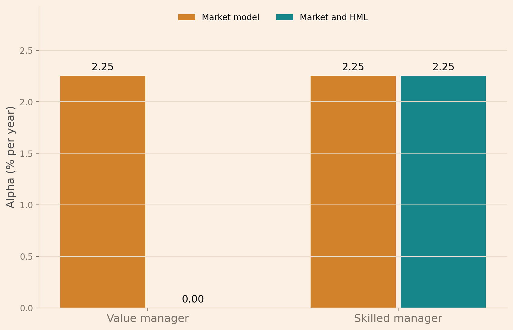
Under the market model, both managers’ portfolios show an alpha of 2.25% per year with a t-statistic of 2.91, so both alphas are statistically different from zero at the 5% significance level. Both of them also have a beta of 0.93. But when I include HML, the value manager’s alpha reduces to 0, its market beta increases to 1, and its HML coefficient is 0.5. In contrast, the skilled manager still has an alpha of 2.25% per year, with a t-statistic of 2.88 and a beta of 0.93.
Including HML does not change the value manager’s portfolio return. It shows that the manager’s supposed alpha comes from its exposure to HML. This result connects back to equation (4), which shows that the intercept takes in part of HML’s average effect.
Step 5. Checking the formulas
I use equations (3) and (4) to cross-check that I get the same answer as when I run the regression. In a sample, the two equations hold exactly for sample averages, variances, and covariances, and for the full regression’s estimated coefficients.
The value manager’s market-model beta is below its true beta of 1 because, in equation (3), HML has a negative slope on the market, since its covariance with the market is negative. With the manager’s positive HML coefficient, the negative slope biases the beta estimate downward when HML is left out.
full = sm.OLS(value, X_full).fit().params
alpha_from_formula = full["const"] + full["HML"] * c
beta_from_formula = full["Mkt-RF"] + full["HML"] * delta
print(f"Market-model alpha {12 * value_market_model.params['const']:.4f}, "
      f"from the formula {12 * alpha_from_formula:.4f} (% per year)")
print(f"Market-model beta {value_market_model.params['Mkt-RF']:.4f}, from the formula {beta_from_formula:.4f}")
Market-model alpha 2.2545, from the formula 2.2545 (% per year)
Market-model beta 0.9298, from the formula 0.9298The output shows that the formulas and the regression give the same alpha and beta for the value manager’s portfolio when HML is left out.
Conclusion
Leaving out factors that could affect the analysis of whether a portfolio manager has skill can bias the conclusion when those factors are relevant. So two managers with the same average return and volatility can show different results when the regression includes factors other than the market’s excess return.
There are also factors other than HML that can be included if a manager’s supposed skill may be an exposure to them, to see whether the alpha is still positive.
An alpha that is not statistically significant is not a verdict that a manager has no skill, because size also matters. Berk and van Binsbergen (2015) find that differences in skill between funds show up mainly in fund size. An alpha in percent can seem large but add less dollar value than a smaller alpha on a larger portfolio.
Read next
- Using the Fama-French factors in Python to test a portfolio’s alpha
- How to use Kenneth French’s data library
- How to calculate abnormal returns for large stocks without bias
Disclaimer: a teaching example on simulated managers, not investment advice.
References
Berk, J. B., & van Binsbergen, J. H. (2015). Measuring skill in the mutual fund industry. Journal of Financial Economics, 118(1), 1–20. https://doi.org/10.1016/j.jfineco.2015.05.002
Fama, E. F., & French, K. R. (1993). Common risk factors in the returns on stocks and bonds. Journal of Financial Economics, 33(1), 3–56. https://doi.org/10.1016/0304-405X(93)90023-5