Currency risk matters, especially if you are Swedish or Swiss

The same S&P 500 total return, 1988 to 2026, converted into six home currencies unhedged, delivered final multiples from 41.1x in Swiss francs to 109.7x in Swedish kronor.

Currency risk matters, especially if you are Swedish or Swiss. The same S&P 500 total return, held from 1988 to 2026 with dividends reinvested, turned one unit into 109.7 times its size for a Swedish investor and 41.1 times for a Swiss one. The dollar investor ended at 65.4 times. The six investors held the identical asset, so the 2.7 times gap between the best and worst outcome is only the exchange rate.

I test whether the currency you count in changes the outcome of a single buy-and-hold investment. I take one series, the S&P 500 total return index, and convert its daily value into six home currencies without hedging: the US dollar, the euro, the yen, the pound, the Swiss franc, and the Swedish krona. The index and the exchange rates come from LSEG, so the raw series stay off this page, and every step of the conversion is here.

What you end up with

• One index. The S&P 500 total return, daily, dividends reinvested, from January 1988.
• Five exchange rates. Daily spot against the dollar for the euro, yen, pound, franc, and krona.
• Six rebased curves. The value of one unit in each home currency, each starting at exactly 1.0.
• A risk table. Final multiple, annual return, annual volatility, and worst drawdown for each currency.

Starting point

The conversion runs off one price file: the index in dollars and one daily spot rate for each currency. Building it is a separate job that depends on the data vendor. I pull from LSEG Workspace. Because the data is licensed, the raw file stays off this page, and I show the code without running it here. The index is the total return series, .SPXTR, which reinvests dividends gross of withholding tax. The official series starts on 4 January 1988, so the October 1987 crash sits just before the sample.

Step 1. One asset, six currencies

Each currency needs one exchange rate and a rule for which way to apply it. Some pairs are quoted as dollars per home unit, and some as home units per dollar, so the conversion divides for the first group and multiplies for the second.

# One asset: the S&P 500 total return index, dividends reinvested, daily from 1988.
SPX_RIC = ".SPXTR"                          # LSEG code for the total return index

# Each FX pair: RIC -> (column name, currency, quoted as USD per home unit?)
FX_PAIRS = {
    "EUR=": ("EURUSD", "EUR", True),        # USD per 1 EUR, so divide; pre-1999 is a synthetic ECU basket
    "JPY=": ("USDJPY", "JPY", False),       # JPY per 1 USD, so multiply
    "GBP=": ("GBPUSD", "GBP", True),        # USD per 1 GBP, so divide
    "CHF=": ("USDCHF", "CHF", False),       # CHF per 1 USD, so multiply
    "SEK=": ("USDSEK", "SEK", False),       # SEK per 1 USD, so multiply
}

A Swedish investor holds a dollar asset, so her krona value is the index times the number of kronor per dollar. The British and euro investors divide instead, because those two rates are quoted as dollars per home unit. The invert flag carries that difference per pair.

Step 2. Convert and rebase

Each day I take the index level in dollars and convert it at that day’s spot rate. Then I rebase every curve to 1.0 at the first common date, so each line reads as the growth of one unit in that currency.

panel = pd.DataFrame({"spxtr": spx})                     # rows are the US index trading days
for name, s in fx.items():                               # add each FX rate as a column
    panel[name] = s.reindex(panel.index).ffill(limit=5)  # align FX, bridge holiday gaps up to 5 days
panel = panel.dropna()                                   # keep dates where the index and every rate exist

home = pd.DataFrame(index=panel.index)
home["USD"] = panel["spxtr"]                             # the US investor holds the raw index
for ric, (name, ccy, invert) in FX_PAIRS.items():        # divide when quoted USD per home unit, else multiply
    home[ccy] = panel["spxtr"] / panel[name] if invert else panel["spxtr"] * panel[name]

idx = home / home.iloc[0]                                # rebase every curve to 1.0 at the common start
print("final multiples:", {k: round(v, 1) for k, v in idx.iloc[-1].items()})

final multiples: {'USD': 65.4, 'EUR': 74.6, 'JPY': 86.3, 'GBP': 92.3, 'CHF': 41.1, 'SEK': 109.7}

The dropna trims the front to 1988, the first date where the index and all five rates exist together. From there the six curves start at the same 1.0 and separate only through the exchange rate.

Step 3. The final multiples and the risk table

For each currency I report the final multiple, the annualised return, the annual volatility, and the deepest drawdown from that curve’s own running peak.

years = (idx.index[-1] - idx.index[0]).days / 365.25     # length of the sample in years
rets  = idx.pct_change().dropna()                        # daily returns of each rebased curve
dd    = idx / idx.cummax() - 1                            # drawdown from each curve's own peak
ann   = idx.iloc[-1] ** (1 / years) - 1                  # annualised return per currency

order   = idx.iloc[-1].sort_values(ascending=False).index
summary = pd.DataFrame({
    "Final multiple":  idx.iloc[-1].map(lambda v: f"{v:,.1f}x"),
    "CAGR":            ann.map(lambda v: f"{v * 100:.1f}%"),
    "Volatility p.a.": (rets.std() * np.sqrt(252)).map(lambda v: f"{v * 100:.1f}%"),
    "Max drawdown":    dd.min().map(lambda v: f"{v * 100:.0f}%"),
}).loc[order]
print(f"S&P 500 total return, {idx.index[0].date()} -> {idx.index[-1].date()} ({years:.1f} years), unhedged")
print(summary.to_string())

S&P 500 total return, 1988-01-04 -> 2026-07-01 (38.5 years), unhedged
    Final multiple   CAGR Volatility p.a. Max drawdown
SEK         109.7x  13.0%           19.1%         -52%
GBP          92.3x  12.5%           19.2%         -52%
JPY          86.3x  12.3%           22.5%         -63%
EUR          74.6x  11.9%           19.9%         -64%
USD          65.4x  11.5%           17.9%         -55%
CHF          41.1x  10.1%           21.8%         -66%

The annual return ranges from 13.0% for the krona down to 10.1% for the franc, with the dollar at 11.5% in between. That is a 2.9 percentage point spread on the same asset. Compounded over 38.5 years, that spread is the whole distance between 109.7 times and 41.1 times.

To see where the spread comes from, I measure how each exchange rate itself drifted over the sample.

fxs      = panel[[name for name, ccy, invert in FX_PAIRS.values()]]   # the raw FX columns
fx_drift = (fxs.iloc[-1] / fxs.iloc[0]) ** (1 / years) - 1            # annualised drift per pair
for name in fxs.columns:
    print(f"{name}: {fx_drift[name] * 100:+.2f}% p.a.")

EURUSD: -0.34% p.a.
USDJPY: +0.72% p.a.
GBPUSD: -0.89% p.a.
USDCHF: -1.20% p.a.
USDSEK: +1.35% p.a.

The krona weakened against the dollar at 1.4% a year, so a Swedish investor earned the dollar return of the index and the currency gain on top. The franc strengthened against the dollar at 1.2% a year, so a Swiss investor earned the same index return minus that currency drag. So, the annual returns in the table line up with the currency drift. The currency that fell against the dollar produced the highest multiple, and the currency that rose produced the lowest.

Results

Growth of one unit in the S&P 500 total return, in six home currencies, 1988 to 2026. All six lines start together at 1.0 and fan out, ending with the Swedish krona highest at 109.7x and the Swiss franc lowest at 41.1x.

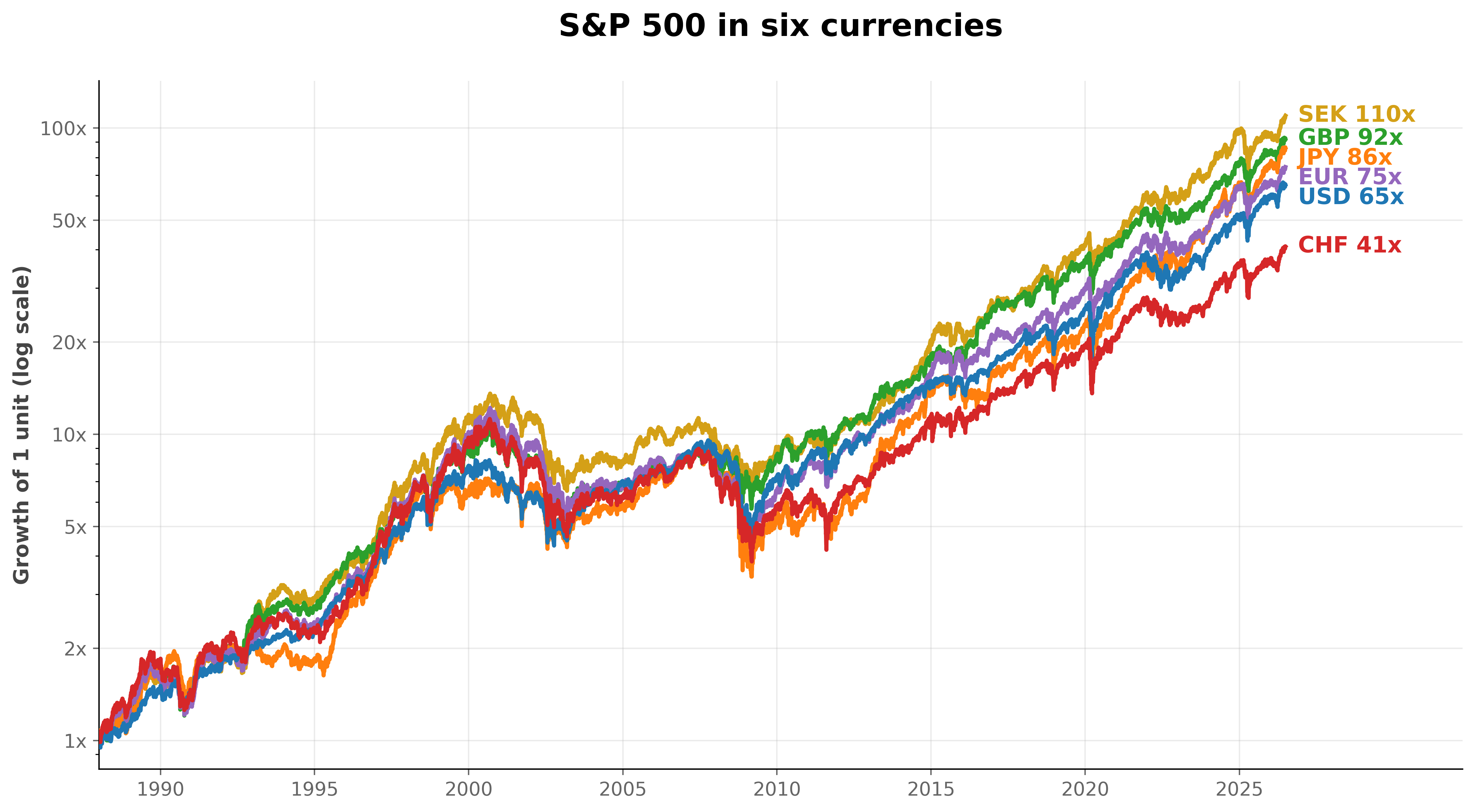
The six lines leave the same point in 1988 and fan out for four decades. The order at the end tracks the exchange rate. The asset was identical for all six. The yen and franc lines were also the most volatile in local terms, at 22.5% and 21.8% a year, against 17.9% for the dollar, because the currency swing adds its own movement to the equity swing. Every investor lived through the same equity crashes, and the currency decided how deep each drawdown ran. The franc tends to strengthen in a crisis, exactly when stocks are falling, so the Swiss investor’s drawdown ran the deepest of the six at 66 percent. The dollar investor’s was 55 percent.

What this test does not settle

The pre-1999 euro is synthetic. The euro did not exist before January 1999, so the early euro line uses LSEG’s ECU-based basket history. Treat the first eleven years of the euro curve as an approximation of a pre-euro basket investor, and the euro multiple as indicative for that stretch.

The Swiss line is the same asset. The franc curve is the identical index, counted in a currency that strengthened against the dollar for four decades. The low multiple is the currency’s story showing through the same asset.

Unhedged, and free of costs and taxes. The conversion applies spot FX with no hedge, no transaction costs, and no withholding on dividends. A hedged investor would sit much closer to the dollar line, so the spread here is the full unhedged case and an upper bound on how much currency can matter.

One index, one span. The test covers the S&P 500 over one mostly rising period and one set of exchange-rate paths. Different currencies, or a span where the dollar strengthened throughout, would reorder the lines. This is one history, and I do not attach a confidence interval to the ranking.

Drawdowns are in local currency. I measure each drawdown from that curve’s own peak in its own currency, so the same crash reads as a different depth per investor. That is the intended lens here, and it is not comparable to a single dollar drawdown.

What it means

The same investment, over the same 38.5 years, ranged from 41.1 times to 109.7 times depending only on the currency the investor counted in. The equity return was identical for all six. The difference is the exchange rate compounding alongside the index, adding to the return where the home currency fell against the dollar and subtracting where it rose. Whether to hedge is a bet on your own currency: over this window it added to the return for the four investors whose currency fell against the dollar and subtracted for the Swiss one, whose currency rose. The takeaway is that the return you earn on a global asset is the asset and the currency together, because the exchange rate compounds over decades just as the price does.

Read next

• Buy the dip? US vs. Europe Another cross-market comparison, this time on when a falling stock is worth buying.
• The Magic Formula worked. Just not lately. A US strategy measured against the same S&P 500 total return used here.

Disclaimer: This is a simplified, hypothetical calculation for discussion purposes only. Not investment advice. Past performance does not predict future returns.

Data: S&P 500 total return index (.SPXTR) and daily spot FX from LSEG Workspace (licensed). I do not reproduce the raw file here.