Why the 10-year Treasury yield near 5% is not a clear warning for stocks
Python
Analysis
Code
After the 10-year Treasury yield was near 5%, the median US stock return over the next year was lower, almost entirely because of 2000 to 2002.
Published
September 15, 2026
All else equal, a higher Treasury yield, the interest rate on US government debt, should lower stock prices, because investors discount future earnings at a higher rate, which makes those earnings worth less today. On 11 September 2026, the 10-year Treasury yield was 4.96%, the highest since 19 October 2023. But have US stocks returned less after the 10-year yield was near 5%?
I compare the US stock return over the 12 months after month-ends when the 10-year yield was near 5%, between 4.5% and 5.5%, with the return after all month-ends from December 1964 to July 2025. The median return, the middle one when the returns are sorted, was 9.3% after the 90 month-ends near 5% and 13.9% after all 728.
So, the issue is that a gap of 4.6 percentage points looks like a warning, and most of it comes from one episode. Without the 20 month-ends near 5% in 2000 to 2002, the median after the other 70 is 13.5%. A test that allows for 12-month returns sharing months finds the full gap statistically different from zero at the 10% level, meaning chance alone would produce it less than 1 time in 10, in only one of the five settings I try.
The data
The comparison needs two daily series, both free to download. The first is the 10-year Treasury yield from FRED, the database of the Federal Reserve Bank of St. Louis, under the code DGS10. The second is the US stock market return from Kenneth French’s data library: the value-weighted return of US common stocks listed on the NYSE, AMEX and Nasdaq, with dividends included, where each stock counts in proportion to its market value. French publishes it as two columns, the market return minus the risk-free rate, the return on a one-month Treasury bill, and the risk-free rate itself, and the code adds the two together.
The code below downloads both files the first time it runs and saves each one as a CSV file, a plain-text table, in the folder the code runs from. Every later run reads the saved files.
import io # io.BytesIO lets pandas read downloaded bytesimport os # os.path.exists checks for a saved fileimport urllib.request # downloads a file from a web addressimport zipfile # opens the zip archive from French's libraryimport numpy as npimport pandas as pdimport matplotlib.pyplot as pltYIELD_CSV ="dgs10_daily.csv"MARKET_CSV ="french_market_daily.csv"FRED_URL ="https://fred.stlouisfed.org/graph/fredgraph.csv?id=DGS10"FRENCH_URL = ("https://mba.tuck.dartmouth.edu/pages/faculty/ken.french/ftp/""F-F_Research_Data_Factors_daily_CSV.zip")def download(url):"""Download the file at url and return its contents as bytes."""# The User-Agent header names the program that asks for the file. Some websites# refuse a request that does not send one. request = urllib.request.Request(url, headers={"User-Agent": "Mozilla/5.0"})with urllib.request.urlopen(request, timeout=300) as response:return response.read()ifnot os.path.exists(YIELD_CSV): fred_bytes = download(FRED_URL)# io.BytesIO wraps the downloaded bytes so that read_csv can read them like a file. fred_file = io.BytesIO(fred_bytes)# na_values="." reads a dot as a missing yield. yields = pd.read_csv(fred_file, na_values=".") yields.columns = ["Date", "DGS10"]# dropna() removes the days without a yield, such as bond-market holidays. yields = yields.dropna()# utf-8-sig starts the file with a marker that tells Excel the text is UTF-8. yields.to_csv(YIELD_CSV, index=False, encoding="utf-8-sig")ifnot os.path.exists(MARKET_CSV): french_bytes = download(FRENCH_URL)# The download is a zip archive that holds one CSV file, and namelist()[0] is its name. french_file = io.BytesIO(french_bytes) archive = zipfile.ZipFile(french_file) csv_name = archive.namelist()[0]# read() gives the CSV file as bytes, and decode("latin-1") turns the bytes into text.# latin-1 can decode every possible byte, so an unusual character cannot stop the code.# splitlines() turns the text into a list with one string per line. csv_bytes = archive.read(csv_name) csv_text = csv_bytes.decode("latin-1") lines = csv_text.splitlines()# The file starts with lines of description. The daily table starts at the first line# that contains the column name Mkt-RF. header_position =0while"Mkt-RF"notin lines[header_position]: header_position = header_position +1# The daily table ends at the first line that does not start with an eight-digit date# such as 19260701. strip() removes spaces at both ends of the line, [:8] keeps the# first eight characters, and isdigit() is True when all eight are digits. break stops# the loop, so the loop leaves out any text after the table. table_lines = [lines[header_position]]for line in lines[header_position +1:]:ifnot line.strip()[:8].isdigit():break table_lines.append(line)# "\n".join puts the lines back together as one text, and io.StringIO lets read_csv# read that text like a file. table_text ="\n".join(table_lines) table_file = io.StringIO(table_text) factors = pd.read_csv(table_file) factors.columns = factors.columns.str.strip() # " Mkt-RF" becomes "Mkt-RF"# The first column holds each date as a number such as 19260701. format="%Y%m%d" tells# to_datetime that the first four digits are the year, then two for the month and two# for the day. date_column = factors.columns[0] date_text = factors[date_column].astype(str) # 19260701 becomes "19260701" date_text = date_text.str.strip() # remove any spaces around it factors["Date"] = pd.to_datetime(date_text, format="%Y%m%d")# Mkt-RF is the market return minus the risk-free rate, and RF is the risk-free rate,# both in percent. Their sum is the market return, and dividing by 100 turns 0.46 into# 0.0046. factors["Mkt"] = (factors["Mkt-RF"] + factors["RF"]) /100 factors[["Date", "Mkt"]].to_csv(MARKET_CSV, index=False, encoding="utf-8-sig")# parse_dates=["Date"] reads the Date column as dates instead of text.yields = pd.read_csv(YIELD_CSV, parse_dates=["Date"], encoding="utf-8-sig")market = pd.read_csv(MARKET_CSV, parse_dates=["Date"], encoding="utf-8-sig")# set_index("Date") makes the dates the row labels. ["DGS10"] then keeps that one column# as a Series, and sort_index() puts the rows in date order.yields = yields.set_index("Date")ten_year_yield = yields["DGS10"]ten_year_yield = ten_year_yield.sort_index()market = market.set_index("Date")daily_return = market["Mkt"]daily_return = daily_return.sort_index()# iloc[-1] is the last value by position, and index[-1] is the date of that value.latest_yield = ten_year_yield.iloc[-1]latest_date = ten_year_yield.index[-1]# iloc[:-1] keeps every day before the last one. Series.loc[condition] keeps the rows where# the condition is True, here the days with a yield at least as high as the latest yield,# and index[-1] is the most recent of those days.earlier_yields = ten_year_yield.iloc[:-1]yields_as_high = earlier_yields.loc[earlier_yields >= latest_yield]last_day_as_high = yields_as_high.index[-1]# In an f-string, :%d %b %Y prints a date as 11 Sep 2026, and :.2f prints two decimals.print(f"10-year yield: {ten_year_yield.index[0]:%d %b %Y} to {latest_date:%d %b %Y}")print(f"stock return: {daily_return.index[0]:%d %b %Y} to {daily_return.index[-1]:%d %b %Y}")print(f"latest 10-year yield: {latest_yield:.2f}% on {latest_date:%d %b %Y}")print(f"last earlier day with a yield of at least {latest_yield:.2f}%: "f"{last_day_as_high:%d %b %Y}")
10-year yield: 02 Jan 1962 to 11 Sep 2026
stock return:  01 Jul 1926 to 31 Jul 2026
latest 10-year yield: 4.96% on 11 Sep 2026
last earlier day with a yield of at least 4.96%: 19 Oct 2023
The yield series starts on 2 January 1962 and the stock series on 1 July 1926. The latest yield in the file is 4.96% on 11 September 2026, and the last earlier day with a yield of at least 4.96% is 19 October 2023.
Returns after each month-end
The two files hold one value per day, and the comparison needs one row per month-end with the stock return 1 to 12 months later. A month-end is the last trading day of a month. The code first turns the daily returns into a total return index, the value of 1 dollar invested at the start of July 1926 with every dividend reinvested. The return from one month-end to a later one is the index at the later month-end divided by the index at the first month-end, minus one.
Each month-end also gets the 10-year yield on the same day, and it counts as near 5% when that yield is between 4.5% and 5.5%, both included. The first month-end is December 1964, the first with three years of yield data, a start date I keep from an earlier version of this analysis that needed three years of yields. The last month-end is July 2025, because the stock file ends on 31 July 2026 and the 12-month return after July 2025 is the last one the file covers.
The code below writes both calculations as functions, return_after for the return from one month-end to a later one and is_yield_near_5 for the band, and checks each function on a small example with a known answer.
FIRST_MONTH ="1964-12"LAST_MONTH ="2025-07"LOWER_YIELD =4.50# near 5% means a yield from 4.50% to 5.50%, both includedUPPER_YIELD =5.50def return_after(index, months_after):"""The return in percent from each row of index to the row months_after rows later. With index [100, 110, 99] and months_after 1, the returns are [10, -10, NaN]: 110 is 10% above 100, 99 is 10% below 110, and the last row has no later row. """# shift(-months_after) moves every value up by months_after rows, so each row holds# the index months_after rows later. index_later = index.shift(-months_after)return100* (index_later / index -1)def is_yield_near_5(yields):"""True for a yield from 4.50% to 5.50%, both included, and False otherwise."""return (yields >= LOWER_YIELD) & (yields <= UPPER_YIELD)# round(10) removes the tiny error of decimal arithmetic in a computer, which gives# 10.000000000000009 instead of 10, and tolist() turns the Series into a plain list.example_index = pd.Series([100.0, 110.0, 99.0])return_after_1_month = return_after(example_index, 1).round(10)return_after_2_months = return_after(example_index, 2).round(10)print(f"example index {example_index.tolist()}")print(f" return after 1 month: {return_after_1_month.tolist()}")print(f" return after 2 months: {return_after_2_months.tolist()}")# FRED reports yields with two decimals, so a yield can be exactly 4.50% or 5.50%.example_yields = pd.Series([4.49, 4.50, 5.00, 5.50, 5.51])example_near_5 = is_yield_near_5(example_yields)print(f"example yields {example_yields.tolist()}, near 5%: {example_near_5.tolist()}")
example index [100.0, 110.0, 99.0]
  return after 1 month:  [10.0, -10.0, nan]
  return after 2 months: [-1.0, nan, nan]
example yields [4.49, 4.5, 5.0, 5.5, 5.51], near 5%: [False, True, True, True, False]
The index of 100, 110 and 99 gives returns of +10% and −10% after one month and −1% after two months, and the yields of 4.50% and 5.50% both count as near 5%. The code below applies both functions to the real data.
# cumprod multiplies (1 + return) day after day, so total_return_index is the value of# 1 dollar invested at the start of the file after each day, with dividends reinvested.total_return_index = (1+ daily_return).cumprod()# to_period("M") turns each date into its calendar month, such as 2025-07. Grouping the# index by that month and taking tail(1) keeps the last trading day of each month.calendar_month = total_return_index.index.to_period("M")month_end_index = total_return_index.groupby(calendar_month).tail(1)# return_after shifts values by rows. One row is one month only when no calendar month is# missing, so the check compares the number of month-ends with the number of months from# the first month-end to the last.month_end_months = month_end_index.index.to_period("M")months_in_range = pd.period_range(month_end_months[0], month_end_months[-1], freq="M")assertlen(month_end_index) ==len(months_in_range), "a calendar month is missing"# One column per horizon, from 1 to 12 months, each holding the return in percent from# every month-end to the month-end months_after rows later.forward_returns = pd.DataFrame(index=month_end_index.index)for months_after inrange(1, 13): forward_returns[months_after] = return_after(month_end_index, months_after)# Keep the month-ends from December 1964 to July 2025.in_study = ((month_end_months >= pd.Period(FIRST_MONTH, "M"))& (month_end_months <= pd.Period(LAST_MONTH, "M")))forward_returns = forward_returns.loc[in_study]# notna() is True where a return exists, and .all().all() is True only when every# month-end in the study has all 12 returns.assert forward_returns.notna().all().all(), "the stock data ends before July 2026"# asof(dates) gives, for each date, the last yield on or before that date, so a month-end# without a yield on the same day would get the yield of an earlier day. isin is True for# each month-end date that appears among the yield dates.month_end_dates = forward_returns.indexyield_at_month_end = ten_year_yield.asof(month_end_dates)yield_on_same_day = month_end_dates.isin(ten_year_yield.index)near_5 = is_yield_near_5(yield_at_month_end)# near_5.sum() counts the True values. ~ turns True into False and False into True, so# (~yield_on_same_day).sum() counts the month-ends without a yield on the same day.print(f"month-ends {month_end_dates[0]:%b %Y} to {month_end_dates[-1]:%b %Y}: "f"{len(month_end_dates)}")print(f"month-ends with the 10-year yield near 5%: {near_5.sum()}")print(f"month-ends without a yield on the same day: {(~yield_on_same_day).sum()}")
month-ends Dec 1964 to Jul 2025: 728
month-ends with the 10-year yield near 5%: 90
month-ends without a yield on the same day: 0
The study has 728 month-ends, and the 10-year yield was near 5% on 90 of them. Every month-end has a yield on the same day, so no month-end uses the yield of an earlier day.
Two medians
With one row per month-end, I compare the median returns at each horizon, 1 to 12 months after the month-end, over all 728 month-ends and over the 90 near 5%. I use the median so that a few very large or very small returns have little effect on the comparison. A median does not show how often the return was negative, so the code also calculates the share of negative 12-month returns.
# median() works column by column, so each result holds one median per horizon.# forward_returns.loc[near_5] keeps the rows of the month-ends near 5%.median_all = forward_returns.median()median_near_5 = forward_returns.loc[near_5].median()medians = pd.DataFrame({"all month-ends": median_all, "near 5%": median_near_5})medians.index.name ="months after"# float_format="{:.1f}".format prints every decimal number with one decimal.print(medians.to_string(float_format="{:.1f}".format))# twelve_month_return < 0 is True for a negative return. The mean of True and False# values is the share of True values.twelve_month_return = forward_returns[12]negative_all =100* (twelve_month_return <0).mean()negative_near_5 =100* (twelve_month_return.loc[near_5] <0).mean()# :+.1f prints one decimal with a sign, such as -4.6 or +13.0.print(f"\n12-month median return: {median_near_5.loc[12]:.1f}% near 5%, "f"{median_all[12]:.1f}% all month-ends, "f"difference {median_near_5.loc[12] - median_all.loc[12]:+.1f} percentage points")print(f"12-month return negative: {negative_near_5:.1f}% near 5%, "f"{negative_all:.1f}% all month-ends, "f"difference {negative_near_5 - negative_all:+.1f} percentage points")
              all month-ends  near 5%
months after
1                        1.3      1.1
2                        2.3      1.0
3                        3.3      1.6
4                        4.4      2.6
5                        5.4      2.3
6                        6.4      2.8
7                        7.5      4.2
8                        8.8      6.9
9                        9.9      7.1
10                      11.3      8.4
11                      12.8      7.3
12                      13.9      9.3

12-month median return: 9.3% near 5%, 13.9% all month-ends, difference -4.6 percentage points
12-month return negative: 34.4% near 5%, 21.4% all month-ends, difference +13.0 percentage points
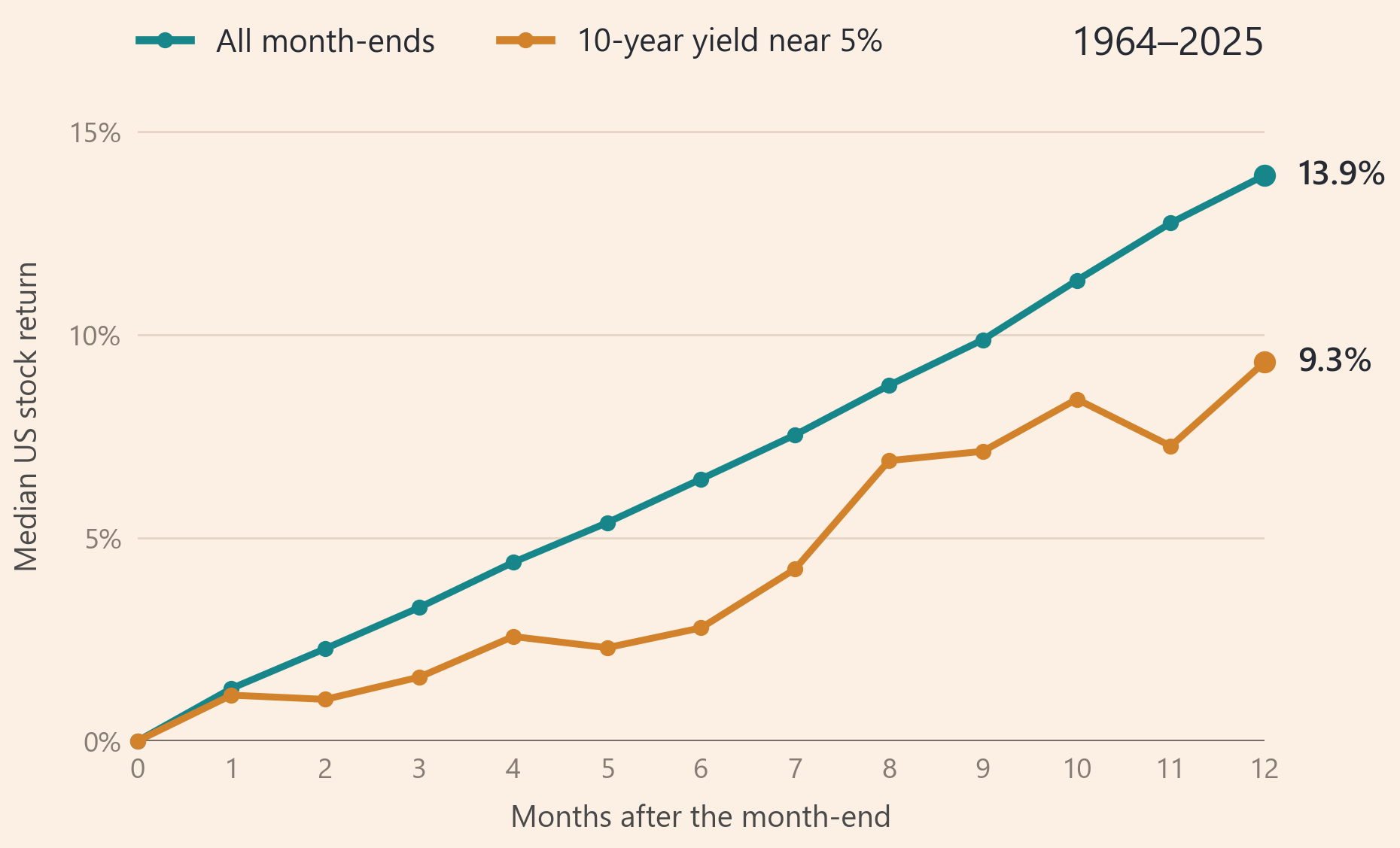
After 12 months, the median return was 9.3% after month-ends near 5% and 13.9% after all month-ends, a difference of −4.6 percentage points. The 12-month return was negative after 34.4% of the month-ends near 5% and after 21.4% of all month-ends, a difference of +13.0 percentage points. The code below plots both medians at every horizon and writes the 12-month median at the end of each line.
import matplotlibfrom matplotlib import font_manager # knows which fonts this computer hasfrom matplotlib.lines import Line2D # a legend entry drawn by hand# matplotlib prints a warning for every requested font it cannot find, so the code first# picks an installed font: Segoe UI, then Arial, and otherwise DejaVu Sans, which comes# with matplotlib.installed_fonts = font_manager.get_font_names()chosen_font ="DejaVu Sans"for font_name in ["Segoe UI", "Arial"]:if font_name in installed_fonts: chosen_font = font_namebreakmatplotlib.rcParams["font.family"] = chosen_fontTEAL, ORANGE ="#17868A", "#D2822B"BACKGROUND, GRID_LINE, ZERO_LINE ="#FCEFE3", "#E6D6C6", "#6f6760"TEXT, LABEL, TICK ="#262a33", "#4a4a4a", "#857c74"# Both lines start at 0% at the month-end itself, horizon 0. [0] + list(...) puts that# zero in front of the 12 medians.horizons = [0] +list(medians.index)all_line = [0] +list(median_all)near_5_line = [0] +list(median_near_5)# all_line + near_5_line joins the two lists into one list of 26 values.# ax.set_ylim(0, 16) below sets the vertical axis from 0% to 16%, so every value has to be# inside that range.lowest_value =min(all_line + near_5_line)highest_value =max(all_line + near_5_line)assert lowest_value >=0and highest_value <=16, "a median is outside the vertical axis"fig, ax = plt.subplots(figsize=(10, 6.25))fig.patch.set_facecolor(BACKGROUND) # the colour around the plotting areaax.set_facecolor(BACKGROUND) # the colour inside the plotting area# The loop runs twice, once per line. Each pass takes one (values, colour, order) group# from the list and stores its three parts in line_values, line_colour and line_order.for line_values, line_colour, line_order in [(all_line, TEAL, 3), (near_5_line, ORANGE, 4)]:# "-o" draws a line with a dot at every horizon. zorder sets the drawing order, so# matplotlib draws the orange line, with the higher zorder, on top of the teal line.# clip_on=False draws the dots at the edge of the plotting area in full. ax.plot(horizons, line_values, "-o", color=line_colour, lw=3.4, ms=7, solid_capstyle="round", zorder=line_order, clip_on=False)# A larger dot at 12 months, and the 12-month median written 0.35 of a month to the# right of that dot.# line_values[-1] is the 12-month median. ax.plot(horizons[-1], line_values[-1], "o", ms=10, color=line_colour, zorder=5, clip_on=False) ax.text(horizons[-1] +0.35, line_values[-1], f"{line_values[-1]:.1f}%", fontsize=17, fontweight="semibold", color=TEXT, va="center", clip_on=False)ax.set_xlim(0, 12)ax.set_ylim(0, 16)ax.set_xticks(horizons)ax.set_yticks([0, 5, 10, 15])ax.set_yticklabels(["0%", "5%", "10%", "15%"])ax.grid(True, axis="y", color=GRID_LINE, lw=1.1)ax.axhline(0, color=ZERO_LINE, lw=1.4, zorder=2) # a darker horizontal line at 0%ax.set_axisbelow(True) # draw the grid lines behind the two lines# ax.spines holds the four borders of the plotting area, and the loop hides all four.for border in ax.spines.values(): border.set_visible(False)# length=0 removes the small tick marks and keeps the tick labels.ax.tick_params(axis="both", length=0, labelsize=14, colors=TICK, pad=8)ax.set_xlabel("Months after the month-end", fontsize=15, color=LABEL, labelpad=10)ax.set_ylabel("Median US stock return", fontsize=15, color=LABEL, labelpad=12)# Two legend entries in one row above the plotting area. bbox_to_anchor=(-0.01, 1.03)# places the lower left corner of the legend at the left edge of the plotting area, just# above its top edge, and ncol=2 puts the two entries side by side.legend_entries = [ Line2D([0], [0], color=TEAL, lw=4, marker="o", ms=7, label="All month-ends"), Line2D([0], [0], color=ORANGE, lw=4, marker="o", ms=7, label="10-year yield near 5%"),]ax.legend(handles=legend_entries, loc="lower left", bbox_to_anchor=(-0.01, 1.03), ncol=2, frameon=False, fontsize=16, handlelength=1.6, columnspacing=2.0, labelcolor=TEXT, borderaxespad=0)# transform=ax.transAxes measures the position as a share of the plotting area: 1.0 is# the right edge and 1.042 is just above the top edge.ax.text(1.0, 1.042, f"{month_end_dates[0]:%Y}–{month_end_dates[-1]:%Y}", transform=ax.transAxes, ha="right", va="bottom", fontsize=20, color=TEXT)# subplots_adjust sets the margins around the plotting area as shares of the figure, which# leaves room for the legend above and the 12-month labels on the right.fig.subplots_adjust(left=0.10, right=0.88, bottom=0.14, top=0.86)plt.savefig("yield_near_5.png", dpi=200, facecolor=BACKGROUND)plt.show()
The teal line is the median return after all month-ends. The orange line is the median return after month-ends near 5%.
So, the median return after month-ends near 5% was lower than the median after all month-ends at every horizon from 1 to 12 months, and it was positive at every horizon. Whether a difference of 4.6 percentage points after 12 months is evidence of lower returns depends on when the 90 month-ends occurred.
The years behind the 90 month-ends
Consecutive month-ends share most of their 12-month returns. The return from the end of January to the end of the next January and the return from the end of February to the end of the next February have 11 months in common, so the stock return in a single month is part of up to twelve 12-month returns. The code below counts the month-ends near 5% in each calendar year, with their median 12-month return and the number of negative 12-month returns.
# One row per month-end near 5%. to_numpy() drops the date labels, so pandas puts each# year and each return in the table by position.near_5_returns = twelve_month_return.loc[near_5]near_5_table = pd.DataFrame({"year": near_5_returns.index.year,"return": near_5_returns.to_numpy(),})near_5_table["negative"] = near_5_table["return"] <0# groupby("year") puts the month-ends of the same year together. count() counts them,# median() takes their median return, and sum() counts their negative returns.grouped = near_5_table.groupby("year")by_year = pd.DataFrame({"month-ends": grouped["return"].count(),"median return (%)": grouped["return"].median(),"negative returns": grouped["negative"].sum(),})print(by_year.to_string(float_format="{:.1f}".format))# loc[[2000, 2001, 2002, 2007], "negative returns"] keeps the counts for those four years.counts_in_four_years = by_year.loc[[2000, 2001, 2002, 2007], "negative returns"]negative_in_four_years = counts_in_four_years.sum()print(f"\n{len(by_year)} years, {by_year['month-ends'].sum()} month-ends, "f"{by_year['negative returns'].sum()} negative 12-month returns")print(f"negative 12-month returns after month-ends in 2000-2002 and 2007: "f"{negative_in_four_years}")
Of the 31 negative 12-month returns after month-ends near 5%, 26 followed month-ends in 2000 to 2002 and 2007. Seventeen negative returns followed the 20 month-ends in 2000 to 2002, and 9 followed the 9 month-ends in 2007. The 12 months after those month-ends include the falls in US stock prices in 2001, 2002 and 2008. The month-ends near 5% in the other 13 of the 17 calendar years account for 5 of the 31.
So, most of the negative 12-month returns after month-ends near 5% come from four of the 17 years, and the 90 month-ends do not give 90 independent 12-month returns. A test of the two differences therefore has to account for 12-month returns that share months and for month-ends near 5% that are concentrated in a few periods.
A block bootstrap
A block bootstrap is one way to account for both. It estimates how much the two differences vary from one sample of month-ends to another, using only the 728 month-ends we have. The code builds a new sample from blocks of consecutive month-ends drawn at random, calculates both differences in the new sample, and repeats this thousands of times.
Say a block has 24 month-ends. A draw picks a random first month-end, such as March 2001, and takes it together with the next 23, so the block ends in February 2003. Each month-end in the block keeps its own 12-month return and its own label, near 5% or not. The draw repeats this for 31 blocks, which gives 744 month-ends, and keeps the first 728, the number of month-ends in the real sample. Some month-ends appear more than once in a draw, and others do not appear at all.
I use 4,000 draws. Each draw that contains at least one month-end near 5% gives one difference in median returns and one difference in the share of negative returns. The 90% interval for a difference is from its 5th percentile to its 95th percentile across the draws, where the 5th percentile is the value with 5% of the draws below it. When zero is inside the 90% interval, the difference is not statistically different from zero at the 10% level.
A block of 24 month-ends keeps two years of consecutive 12-month returns together. Inside a block, 12-month returns that share months stay next to each other, and the boundary between two blocks separates them. Because no rule fixes the block length, the code also runs blocks of 12, 36, 48 and 60 month-ends.
def differences(returns, is_near_5):"""Near 5% minus all month-ends, for the median return and for the share of negative returns, both in percentage points. With returns [-2, 4, 10] and is_near_5 [True, True, False], the median near 5% is 1 and the median of all three returns is 4, so the difference in median returns is -3. """ near_5_returns = returns[is_near_5] median_difference = np.median(near_5_returns) - np.median(returns) negative_difference =100* (np.mean(near_5_returns <0) - np.mean(returns <0))return median_difference, negative_differencedef block_bootstrap_intervals(returns, is_near_5, block_length, draws=4000, seed=65):"""The 90% interval for both differences, from a moving block bootstrap. Each draw builds a new sample from blocks of block_length consecutive month-ends, each block starting at a random month-end, and calculates both differences. Each interval is from the 5th to the 95th percentile of the differences across the draws. """# The same seed gives the same random numbers every time the code runs. generator = np.random.default_rng(seed) number_of_month_ends =len(returns)# np.ceil rounds up, so 728 month-ends in blocks of 24 need 31 blocks, because 30# blocks hold only 720 month-ends. blocks_per_draw =int(np.ceil(number_of_month_ends / block_length)) median_differences = [] negative_differences = []# _ holds the draw number, 0, 1, 2, ..., which the code inside the loop does not use.for _ inrange(draws):# integers(low, high, size) draws size random whole numbers from low to high - 1.# The highest first position is number_of_month_ends - block_length, so the last# block the code can draw ends at the last month-end. block_starts = generator.integers(0, number_of_month_ends - block_length +1, size=blocks_per_draw)# extend adds every position in one block to the list, such as 100 to 123 for a# block of 24 that starts at position 100. positions = []for start in block_starts: positions.extend(range(start, start + block_length)) positions = positions[:number_of_month_ends] # as many as the month-ends sample_returns = returns[positions] sample_is_near_5 = is_near_5[positions]# A sample without any month-end near 5% has no median near 5%, so the code skips# that sample. any() is True when at least one value is True.if sample_is_near_5.any(): median_difference, negative_difference = differences(sample_returns, sample_is_near_5) median_differences.append(median_difference) negative_differences.append(negative_difference)# np.percentile(values, [5, 95]) returns the 5th and the 95th percentile of values. median_low, median_high = np.percentile(median_differences, [5, 95]) negative_low, negative_high = np.percentile(negative_differences, [5, 95])return median_low, median_high, negative_low, negative_high# returns[positions] inside the function selects values by a list of positions, which# works on the numpy arrays that to_numpy() gives.returns = twelve_month_return.to_numpy()is_near_5 = near_5.to_numpy()median_difference, negative_difference = differences(returns, is_near_5)print(f"difference in median returns: {median_difference:+.2f} percentage points")print(f"difference in share of negative returns: {negative_difference:+.2f} percentage points")print("\n90% intervals, in percentage points")for block_length in [24, 12, 36, 48, 60]: median_low, median_high, negative_low, negative_high = block_bootstrap_intervals( returns, is_near_5, block_length)# median_low <= 0 <= median_high is True when zero is inside the interval. median_has_zero = median_low <=0<= median_high negative_has_zero = negative_low <=0<= negative_highprint(f"blocks of {block_length}: "f"median [{median_low:+.2f}, {median_high:+.2f}] zero inside: {median_has_zero}; "f"negative share [{negative_low:+.2f}, {negative_high:+.2f}] "f"zero inside: {negative_has_zero}")
difference in median returns:           -4.60 percentage points
difference in share of negative returns: +13.02 percentage points

90% intervals, in percentage points
blocks of 24: median [-19.97, +0.56] zero inside: True; negative share [-5.51, +33.66] zero inside: True
blocks of 12: median [-17.36, +0.16] zero inside: True; negative share [-3.98, +30.63] zero inside: True
blocks of 36: median [-21.61, +0.28] zero inside: True; negative share [-4.64, +36.66] zero inside: True
blocks of 48: median [-21.78, +0.01] zero inside: True; negative share [-2.61, +35.60] zero inside: True
blocks of 60: median [-21.28, -0.40] zero inside: False; negative share [-1.68, +34.39] zero inside: True
With blocks of 24 month-ends, the 90% interval for the difference in median returns is from −19.97 to +0.56 percentage points. The 90% interval for the difference in the share of negative returns is from −5.51 to +33.66 percentage points. Both intervals contain zero, so neither difference is statistically different from zero at the 10% level.
The upper end of the interval for the difference in median returns, +0.56, is close to zero, and the conclusion depends on the block length. With blocks of 12, 36 and 48 month-ends, the interval for the difference in median returns also contains zero, and with blocks of 48 its upper end is +0.01. With blocks of 60 month-ends, the interval is from −21.28 to −0.40, and it does not contain zero. The interval for the difference in the share of negative returns contains zero at all five block lengths.
Without 2000 to 2002
The per-year counts showed that 17 of the 31 negative 12-month returns followed the 20 month-ends near 5% in 2000 to 2002. The code below removes those 20 month-ends from the month-ends near 5% and calculates the median 12-month return after the other 70.
# month_end_dates.year gives the year of every month-end, and isin([2000, 2001, 2002]) is# True for the month-ends in those three years, so near_5_outside_2000_2002 is True for a# month-end near 5% in any other year.in_2000_2002 = month_end_dates.year.isin([2000, 2001, 2002])near_5_outside_2000_2002 = near_5 &~in_2000_2002median_outside = twelve_month_return.loc[near_5_outside_2000_2002].median()print(f"month-ends near 5% outside 2000-2002: {near_5_outside_2000_2002.sum()} "f"of {near_5.sum()}")print(f"12-month median return: {median_outside:.1f}% near 5% outside 2000-2002, "f"{median_all[12]:.1f}% all month-ends, "f"difference {median_outside - median_all.loc[12]:+.1f} percentage points")
month-ends near 5% outside 2000-2002: 70 of 90
12-month median return: 13.5% near 5% outside 2000-2002, 13.9% all month-ends, difference -0.5 percentage points
Without the month-ends in 2000 to 2002, the median 12-month return after month-ends near 5% is 13.5%, against 13.9% after all month-ends, which is unchanged because the code removes the 20 month-ends from the month-ends near 5% only. So, removing the month-ends of three of the 17 years reduces the gap from 4.6 to 0.5 percentage points.
Limitations
The comparison does not isolate the 10-year yield. Inflation, Federal Reserve interest rates and company earnings can change at the same time as the 10-year yield. Because the comparison holds none of them fixed, it does not measure the effect of the 10-year yield on stock returns.
Near 5% is one band. A month-end counts as near 5% when the yield is between 4.5% and 5.5%. I do not vary the band, and a narrower or a wider band includes a different set of month-ends.
The label uses only the level of the yield. A month-end with a yield of 5% after an increase from 4% counts the same as a month-end with a yield of 5% after a decrease from 6%.
Conclusion
From 1964 to 2025, a 10-year yield near 5% preceded a lower median 12-month return, 9.3% against 13.9%, but the median return was still positive. Whether the difference in median returns is statistically different from zero at the 10% level depends on the block length, and the difference in the share of negative returns is not statistically different from zero at any of the five block lengths.
The takeaway is that a 10-year yield near 5% was not a clear warning for stocks from 1964 to 2025, because the evidence for a lower median return depends on the block length and comes mostly from the month-ends of 2000 to 2002.
Read next
Why the 60/40 portfolio is not dead. Another conclusion drawn from a few years of returns, and how the sample period and the return interval change it.
Disclaimer: a teaching example, not investment advice.
Sources: Board of Governors of the Federal Reserve System, Market Yield on U.S. Treasury Securities at 10-Year Constant Maturity (DGS10), retrieved from FRED, Federal Reserve Bank of St. Louis. Kenneth R. French, Data Library, Fama/French 3 Factors, daily.