In a simulation, a daily loss forecast exceeded on 5% of all days, as intended, is exceeded on 20% of volatile days.
Published
September 22, 2026
Every evening, we forecast a threshold for our portfolio’s loss on the next day, a level that the loss should exceed with a probability of only 5%. A forecast of 1.74% says that the portfolio loses more than 1.74% of its value the next day with a probability of 5%. We choose the 5%, and a forecast rule estimates the threshold from past returns.
I simulate a market in which calm periods alternate with volatile periods of larger daily moves. A fixed rule forecasts the same threshold every day, 1.74%, the loss exceeded on 5% of 2,000 past days. Over the next 2,000 days, the loss is above 1.74% on 5.1% of the days, close to the intended 5%, but on 1.3% of the calm days and 20.2% of the volatile days. The fixed threshold is too high on calm days and too low on volatile days, and over all days the two errors cancel, because calm days are four times as common as volatile days.
Validating a forecast means checking that it is fit for its intended use. I validate the fixed rule in three steps: state the intended use, test the rule on days it was not fitted on, and ask whether its errors matter for that use.
Step 1: Stating the intended use
The first step states what the forecast is and what it is for, because the use decides which errors matter. The daily return \(r_t\) is the percentage change in the portfolio’s value on day \(t\), and the daily loss is \(L_t = -r_t\), so a return of −2% is a loss of 2%, and a gain is a negative loss. The forecast for day \(t\) is a threshold set at the close of day \(t-1\), and a correct forecast satisfies
\[P(L_t > \text{threshold}_t \mid \text{information available before day } t) = 5\%,\]
where \(P\) is a probability and the vertical bar means “given”. So the 5% has to hold on each day, given what we know the evening before, including whether recent days were volatile. The fixed rule in the opening is exceeded on 5% of all days and still fails this. The threshold is also called the 95% one-day value at risk, because the loss is at or below it with a probability of 95%. A day with a loss above that day’s threshold is an exceedance.
We compare each forecast with a limit that we choose, the largest forecast loss we accept. If the forecast is above the limit, we sell some risky investments for cash, which lowers the portfolio’s risk. I validate the forecasts for an unchanged portfolio and do not simulate these sales.
Simulating the data
The other two steps need a history of daily returns, so I simulate 4,000 trading days. Each forecast rule below estimates one number from the first 2,000 days, the fitting sample, and I test the rules on the last 2,000 days, the test sample. Each half has two volatile periods of 200 days, so 400 volatile days and 1,600 calm days. Day \(t\)’s return is
\[r_t = \sigma_t\, z_t,\]
where \(\sigma_t\) is the standard deviation of the return, a measure of how far returns typically are from their mean: 0.8% on a calm day and 2.0% on a volatile day. Each \(z_t\) is a draw from the standard normal distribution, which is bell-shaped with a mean of 0 and a standard deviation of 1. The two standard deviations, 0.8% and 2.0%, and the volatile periods are assumptions. The draws are independent from day to day: one day’s draw says nothing about the next day’s.
The loss \(L_t = -\sigma_t z_t\) is above \(1.645\,\sigma_t\) exactly when \(z_t\) is below −1.645, and a standard normal draw is below −1.645 with a probability of 5%:
Each day’s true threshold is therefore \(1.645\,\sigma_t\): 1.645 × 0.8% = 1.32% on a calm day and 1.645 × 2.0% = 3.29% on a volatile day. I know it because I set \(\sigma_t\); with real data it is unknown. The box below has the code that simulates the returns.
NoteHow the returns are simulated
The block below simulates the returns, marks the fitting sample and the test sample, and computes the true threshold on a calm and on a volatile day.
import numpy as npimport pandas as pdfrom scipy.stats import normN_DAYS =4000# trading days in the simulationN_FITTING =2000# fitting sample: days 1 to 2,000; the rest is the test sampleCALM_SD =0.8# standard deviation of a calm day's return, in percentVOLATILE_SD =2.0# standard deviation of a volatile day's return, in percent# The first and last day of each volatile period; every other day is calmVOLATILE_PERIODS = [(401, 600), (1401, 1600), (2401, 2600), (3401, 3600)]# rng is NumPy's random number generator. Starting it from a fixed number, the seed 923,# gives the same random numbers on every run, so every number in the post reproduces.rng = np.random.default_rng(923)# RangeIndex numbers the days 1 to 4,000 and uses those numbers as the row labelsdays = pd.RangeIndex(1, N_DAYS +1, name="day")# A Series is one column of values with a label for each row. is_volatile starts as False on# every day, and the loop sets the days of each volatile period to True.is_volatile = pd.Series(False, index=days)for first_day, last_day in VOLATILE_PERIODS:# .loc selects rows by label, and a label slice such as 401:600 includes both ends is_volatile.loc[first_day:last_day] =True# each day's standard deviation, first the calm value on every daydaily_sd = pd.Series(CALM_SD, index=days)# .loc with a True/False Series selects the rows marked True, here the volatile daysdaily_sd.loc[is_volatile] = VOLATILE_SD# standard_normal gives normally distributed numbers with a mean of 0 and a standard deviation# of 1, so multiplying them by daily_sd gives each day's return that day's standard deviationreturns = daily_sd * rng.standard_normal(N_DAYS)fitting_sample = days <= N_FITTING # True on days 1 to 2,000test_sample =~fitting_sample # ~ turns True into False and False into True# True counts as 1 and False as 0, so sum() counts the days marked True. An f-string, f"...",# fills in the value of each expression in braces: {x:,} writes x with commas between# thousands, and {x:.2f} with two decimals.print(f"fitting sample: {fitting_sample.sum():,} days, "f"{is_volatile.loc[fitting_sample].sum()} of them volatile")print(f"test sample: {test_sample.sum():,} days, "f"{is_volatile.loc[test_sample].sum()} of them volatile")# norm.ppf(0.95) is 1.645, the value that a standard normal draw is below with a probability of# 95%. By symmetry, a draw is below -1.645 with a probability of 5%.Z_95 = norm.ppf(0.95)print(f"true 95% daily loss threshold on a calm day: {Z_95 * CALM_SD:.2f}%")print(f"true 95% daily loss threshold on a volatile day: {Z_95 * VOLATILE_SD:.2f}%")
fitting sample: 2,000 days, 400 of them volatile
test sample:    2,000 days, 400 of them volatile
true 95% daily loss threshold on a calm day:     1.32%
true 95% daily loss threshold on a volatile day: 3.29%
Defining two forecast rules
I compare the fixed rule, which uses the same threshold every day, with an adaptive rule, which sets a higher threshold when recent returns are more variable. Both rules use only past returns, never the \(\sigma_t\) I set. The adaptive rule is a benchmark: it shows whether the same past returns can give a better threshold.
The fixed threshold is the 95th percentile \(Q_{95}\) of the fitting-sample losses, the loss that 95% of them are at or below:
The adaptive threshold has the form of the true threshold, \(1.645\,\sigma_t\), a multiplier times the day’s standard deviation, and estimates both parts from past returns:
\[\text{adaptive threshold}_t = k\,\hat\sigma_t, \qquad \hat\sigma_t = \operatorname{sd}(r_{t-20}, \dots, r_{t-1}), \qquad k = Q_{95}(L_t/\hat\sigma_t \text{ in the fitting sample}).\]
The recent volatility \(\hat\sigma_t\), where the hat marks an estimate, is the standard deviation (sd) of the 20 returns before day \(t\), about one month of trading, so it never uses the return of day \(t\) itself. Dividing each fitting-sample loss by that day’s recent volatility puts calm and volatile days on one scale: a 2% loss at a recent volatility of 2% and a 0.8% loss at 0.8% both become 1. The multiplier \(k\), the 95th percentile of these scaled losses, takes the place of 1.645. The block below computes both thresholds for every day.
WINDOW =20# trading days in the recent volatility, about one monthdef forecast_thresholds(returns):"""Compute the fixed and the adaptive 95% daily loss threshold for every day. The fixed threshold and the multiplier come from the fitting sample. For a test-sample day, the forecast uses returns up to the day before it. Returns, losses and thresholds are in percent. """ loss =-returns # the loss is minus the return, so a gain is a negative loss# a table whose first column is the loss, with the days as row labels forecasts = pd.DataFrame({"loss": loss})# Fixed rule: quantile(0.95) is the 95th percentile of the fitting-sample losses, used on# every day forecasts["fixed threshold"] = loss.loc[fitting_sample].quantile(0.95)# Adaptive rule. rolling(20).std() on day t is the standard deviation of the returns on# days t-19 to t, which includes day t itself. shift(1) moves every value one row down,# so the value on day t becomes the standard deviation of days t-20 to t-1, which is# known at the close of day t-1. forecasts["recent volatility"] = returns.rolling(WINDOW).std().shift(1)# The loss in units of recent volatility. The first 20 days have no recent volatility,# so their scaled loss is missing (NaN), and quantile() skips missing values. scaled_loss = loss / forecasts["recent volatility"]# the multiplier, the 95th percentile of the fitting-sample scaled losses, on every row forecasts["multiplier"] = scaled_loss.loc[fitting_sample].quantile(0.95) forecasts["adaptive threshold"] = forecasts["multiplier"] * forecasts["recent volatility"]return forecastsforecasts = forecast_thresholds(returns)# The fixed threshold and the multiplier are the same on every row, so the first row shows# them. .iloc selects by position, so .iloc[0] is the first row, day 1, and# .loc[2500, column] selects the row labelled 2500 and one column.print(f"fixed threshold, every day: {forecasts['fixed threshold'].iloc[0]:.3f}%")print(f"multiplier, every day: {forecasts['multiplier'].iloc[0]:.3f}")print(f"day 2,500: recent volatility {forecasts.loc[2500, 'recent volatility']:.3f}%, "f"adaptive threshold {forecasts.loc[2500, 'adaptive threshold']:.3f}%")
fixed threshold, every day: 1.740%
multiplier, every day:      1.801
day 2,500: recent volatility 2.002%, adaptive threshold 3.606%
The fixed threshold is 1.740%, between the true thresholds of 1.32% and 3.29%, because it is estimated on a mix of 80% calm and 20% volatile days. The multiplier is 1.801, above 1.645, because a recent volatility from only 20 returns is sometimes too low, and dividing by it gives some scaled losses that are too large. On day 2,500, in a volatile period of the test sample, the recent volatility is 2.002%, so the adaptive threshold is 1.801 × 2.002% = 3.606%, against a true threshold of 3.29%.
Step 2: Testing on unused days
The second step counts each threshold’s exceedances on the 2,000 test days, which neither rule was fitted on, over all test days and separately on calm and on volatile days, because our use needs a correct threshold on both kinds of day. Even a correct threshold is not exceeded on exactly 5% of days. If each day has a 5% probability of an exceedance, independently of the other days, the number of exceedances \(X\) in a group of \(n\) days follows a binomial distribution, the distribution of a count of independent events that each have the same probability:
where \(\sim\) means “follows” and \(\mathrm{E}[X]\) is the expected number of exceedances, such as 0.05 × 400 = 20 on the 400 volatile days. In the table below, the column “range if correct” runs from the 2.5th to the 97.5th percentile of this distribution, so a correct threshold’s count is inside it with a probability of about 95%. A threshold passes the count check for a group of days if its count is inside that range. The columns fixed and adaptive count each threshold’s exceedances, and the % columns give them as shares of the group’s days.
from scipy.stats import binom# .copy() makes test a separate table, so pandas does not warn when columns are added to ittest = forecasts.loc[test_sample].copy()test["fixed exceeded"] = test["loss"] > test["fixed threshold"]test["adaptive exceeded"] = test["loss"] > test["adaptive threshold"]test_is_volatile = is_volatile.loc[test_sample]# The three groups of test days in the table. items() gives each group's name and table.groups = {"all test days": test,"calm days": test.loc[~test_is_volatile],"volatile days": test.loc[test_is_volatile]}rows = []for name, group in groups.items(): n_days =len(group)# If a threshold is correct, its number of exceedances in n_days days follows a binomial# distribution with a 5% probability each day. binom.ppf(0.025, ...) and# binom.ppf(0.975, ...) leave at most a 2.5% probability of a count below the first or# above the second, so a correct threshold's count is between them with a probability of# about 95% lowest = binom.ppf(0.025, n_days, 0.05) highest = binom.ppf(0.975, n_days, 0.05) rows.append({"group": name,"days": n_days,"expected": 0.05* n_days,"range if correct": f"{lowest:.0f} to {highest:.0f}","fixed": group["fixed exceeded"].sum(),"fixed %": 100* group["fixed exceeded"].sum() / n_days,"adaptive": group["adaptive exceeded"].sum(),"adaptive %": 100* group["adaptive exceeded"].sum() / n_days})# set_index makes the group names the row labels, and round(1) shows one decimalexceedance_table = pd.DataFrame(rows).set_index("group")print(exceedance_table.round(1).to_string())
               days  expected range if correct  fixed  fixed %  adaptive  adaptive %
group
all test days  2000     100.0        81 to 120    102      5.1        96         4.8
calm days      1600      80.0         63 to 97     21      1.3        72         4.5
volatile days   400      20.0         12 to 29     81     20.2        24         6.0
On the 400 volatile days, the fixed threshold is exceeded on 81 days, against 20 expected and above the range of 12 to 29. On the 1,600 calm days, it is exceeded on 21, against 80 expected and below the range of 63 to 97. Over all 2,000 test days, the 61 extra exceedances on volatile days and the 59 missing on calm days almost cancel: 102 exceedances, inside the range of 81 to 120. So the fixed threshold passes the count check over all test days and fails it on calm and on volatile days.
The adaptive threshold’s counts, 96 over all test days, 72 on calm days and 24 on volatile days, are inside all three ranges. A count inside its range can still include weeks with too many exceedances, so a timeline shows on which days the exceedances happen.
Plotting when the exceedances happen
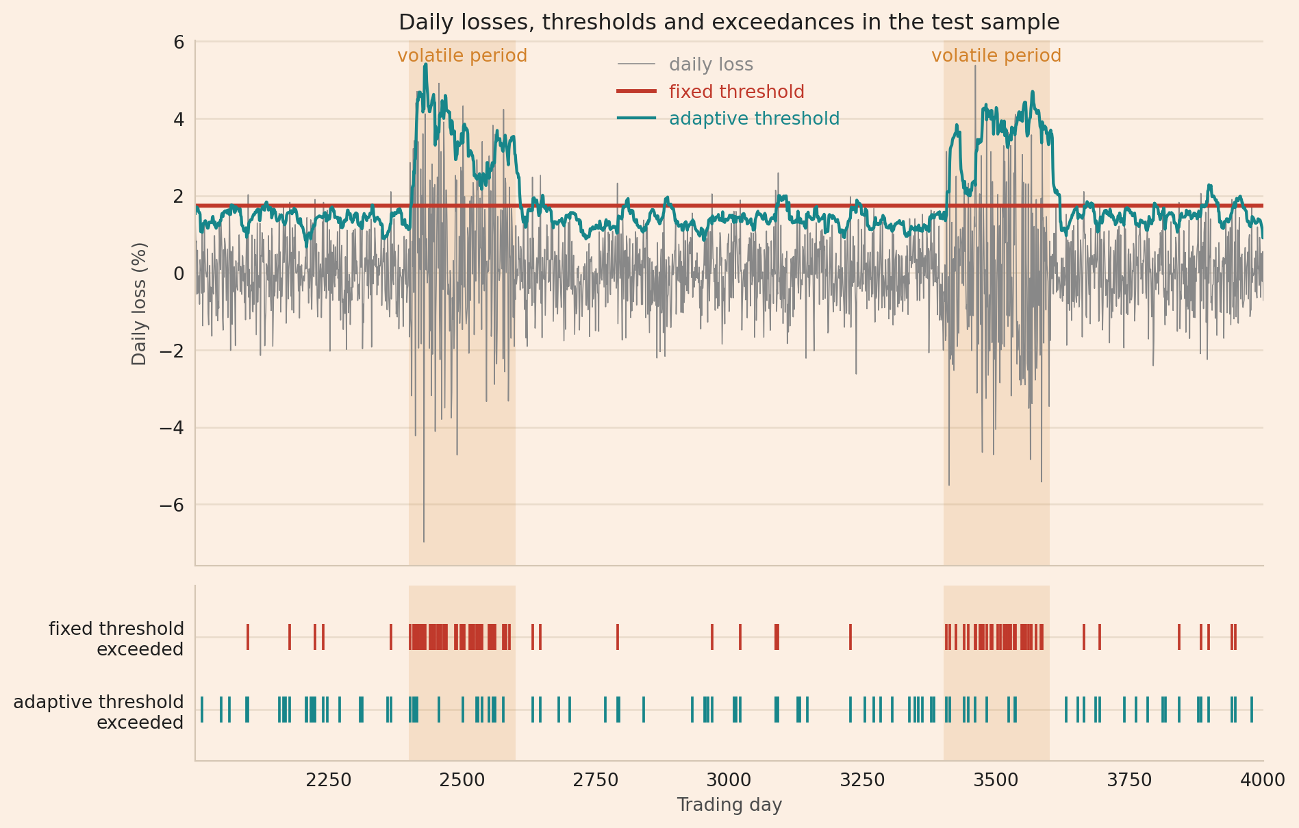
The chart below is a timeline of the test sample. The chart’s top panel plots each test day’s loss in grey, the fixed threshold in red and the adaptive threshold in teal, with the two volatile periods shaded. The bottom panel marks each exceedance in the colour of its threshold. The chart’s code also counts the exceedances in each volatile period and in its first 20 days.
Show the chart code
import matplotlib.pyplot as pltRED, TEAL, ORANGE, GREY ="#C0392B", "#17868A", "#D2822B", "#888888"# The site's chart colours, in order: the cream background, the text, the light grid lines,# the pale frame and the axis labels, the same on every chart of the site.BG, INK, GRID, SPINE, AXIS_TEXT ="#FCEFE3", "#1f1f1f", "#EADCCC", "#D5C6B4", "#4a4a4a"def style_chart(figure, axis):"""Give a finished chart the site's cream background, light grid and pale frame.""" figure.patch.set_facecolor(BG) axis.set_facecolor(BG) axis.grid(True, axis="y", color=GRID, lw=1.0) axis.set_axisbelow(True)for side in ("top", "right"): axis.spines[side].set_visible(False)for side in ("left", "bottom"): axis.spines[side].set_color(SPINE) axis.tick_params(axis="both", length=0, colors=INK, pad=6) axis.xaxis.label.set_color(AXIS_TEXT) axis.yaxis.label.set_color(AXIS_TEXT) axis.title.set_color(INK)# Write each legend entry in the colour of what it labels: a line's colour or a bar's fill# colour. get_legend() returns None when the chart has no legend. legend = axis.get_legend()if legend isnotNone:for text, handle inzip(legend.get_texts(), legend.legend_handles):ifhasattr(handle, "get_color"): text.set_color(handle.get_color())else: text.set_color(handle.get_facecolor())# Two panels that share the day axis: the losses and thresholds on top, and below them one# row of marks for each threshold, with a mark on each day the threshold was exceeded.# figsize is the figure's width and height in inches, and height_ratios makes the top panel# three times as tall as the bottom one.figure, (loss_axis, exceedance_axis) = plt.subplots(2, 1, figsize=(10, 6.4), sharex=True, gridspec_kw={"height_ratios": [3, 1]})# Shade the two volatile periods of the test sample on both panels. alpha=0.15 makes the# shading mostly transparent, and lw, the line width, is 0, so the shading has no edge line.for first_day, last_day in VOLATILE_PERIODS:if first_day > N_FITTING: loss_axis.axvspan(first_day, last_day, color=ORANGE, alpha=0.15, lw=0) exceedance_axis.axvspan(first_day, last_day, color=ORANGE, alpha=0.15, lw=0)# a label above each shaded period, at the height of the largest test-sample loss loss_axis.text((first_day + last_day) /2, test["loss"].max(), "volatile period", ha="center", va="bottom", color=ORANGE)loss_axis.plot(test.index, test["loss"], color=GREY, lw=0.6, label="daily loss")loss_axis.plot(test.index, test["fixed threshold"], color=RED, lw=2.2, label="fixed threshold")loss_axis.plot(test.index, test["adaptive threshold"], color=TEAL, lw=1.6, label="adaptive threshold")loss_axis.set_ylabel("Daily loss (%)")loss_axis.set_title("Daily losses, thresholds and exceedances in the test sample")# the legend lists each line's label; frameon=False draws it without a box, and loc puts it at# the top centre, between the volatile periodsloss_axis.legend(frameon=False, loc="upper center")style_chart(figure, loss_axis)# "|" draws a short vertical mark on each exceedance day, at height 1 for the fixed# threshold and at height 0 for the adaptive threshold. ms sets the mark's length and mew its# line width.fixed_exceedance_days = test.loc[test["fixed exceeded"]].indexadaptive_exceedance_days = test.loc[test["adaptive exceeded"]].indexexceedance_axis.plot(fixed_exceedance_days, np.ones(len(fixed_exceedance_days)), "|", color=RED, ms=14, mew=1.4)exceedance_axis.plot(adaptive_exceedance_days, np.zeros(len(adaptive_exceedance_days)), "|", color=TEAL, ms=14, mew=1.4)# label the two rows of marks at heights 0 and 1, and set the ranges shown on the two axesexceedance_axis.set_yticks([0, 1], ["adaptive threshold\nexceeded", "fixed threshold\nexceeded"])exceedance_axis.set_ylim(-0.7, 1.7)exceedance_axis.set_xlim(N_FITTING +1, N_DAYS)exceedance_axis.set_xlabel("Trading day")style_chart(figure, exceedance_axis)# tight_layout() fits the labels inside the figure. savefig writes the chart to a PNG file:# dpi=140 sets its resolution, bbox_inches="tight" trims the empty margin, and facecolor=BG# keeps the cream background. show() displays the chart.plt.tight_layout()plt.savefig("exceedance_timeline.png", dpi=140, bbox_inches="tight", facecolor=BG)plt.show()# Count the exceedances inside each volatile period of the test sample, and the adaptive# threshold's exceedances in the period's first 20 days, when the recent volatility still# includes returns from calm days. A .loc label slice includes both ends, so first_day to# first_day + WINDOW - 1 is 20 days.for first_day, last_day in VOLATILE_PERIODS:if first_day > N_FITTING: period = test.loc[first_day:last_day] first_20_days = test.loc[first_day:first_day + WINDOW -1]print(f"days {first_day:,} to {last_day:,}: fixed threshold exceeded on "f"{period['fixed exceeded'].sum()} days, adaptive threshold on "f"{period['adaptive exceeded'].sum()}, "f"{first_20_days['adaptive exceeded'].sum()} of them in the first {WINDOW} days")
days 2,401 to 2,600: fixed threshold exceeded on 47 days, adaptive threshold on 15, 6 of them in the first 20 days
days 3,401 to 3,600: fixed threshold exceeded on 34 days, adaptive threshold on 9, 2 of them in the first 20 days
Most red marks are inside the two shaded periods, so the fixed threshold is exceeded mostly on volatile days. The teal marks are spread over the whole test sample, except for a cluster at the start of the first shaded period.
The printed lines split the exceedances on volatile days between the two volatile periods of the test sample: 47 and 34 of the fixed threshold’s 81, and 15 and 9 of the adaptive threshold’s 24. They also show the adaptive threshold’s weak spot. In the first 20 days of the two volatile periods, 40 days in all, the loss is above the adaptive threshold on 6 + 2 = 8 days, 20% of the 40, and on the other 360 volatile days on 16, 4.4% of the 360. At the start of a volatile period, the 20 returns behind the recent volatility still include calm days, so the adaptive threshold is too low.
Step 3: Judging whether the errors matter
The third step asks what the fixed threshold’s errors mean for our use. Say the limit is 1.74%, the same as the fixed forecast. The forecast is then never above the limit, so we never sell, although on a volatile day the true threshold is 3.29%, 3.29/1.74 = 1.9 times the limit. So in volatile periods we keep more risk than the limit allows.
The action that follows is to develop a rule that adjusts to recent volatility, such as the adaptive rule, and to validate that rule with the same three steps before it replaces the fixed rule. In that validation, we have to check the first 20 days of each volatile period, when the adaptive threshold was exceeded on 20% of those days.
Limitations
The simulation labels the periods. Real returns come without labels for calm and volatile days, so a test has to group days by a condition known before each day, such as the recent volatility. Grouping days by their own loss would put the exceedances in the high-loss group automatically, whatever the forecast.
Both samples have the same share of volatile days. With real data the shares may differ. A fixed threshold then tends to be exceeded on less than 5% of the days of a test sample calmer than the fitting sample, and on more than 5% of the days of a more volatile one.
An exceedance count ignores the size of the loss. Against a threshold of 1.74%, a loss of 1.8% and a loss of 7% count as one exceedance each, so we also need to check how large the losses above the threshold are.
Counts are one check among several. Before trusting any count, we check that no return is missing, that the returns are in the unit the forecast expects, and that each forecast uses only returns known the evening before its day. We also check whether losses above the threshold occur on consecutive days more often than a probability of 5% on each day implies.
Conclusion
The takeaway is that a loss forecast can be exceeded on 5% of all days and still be inaccurate on both calm and volatile days, so a loss forecast has to be tested separately in each condition that matters for its use.
Read next
What AUC misses about predicted probabilities The same problem for predicted probabilities: expected and observed crimes can agree over all announcements while the probabilities are too high in some groups and too low in others.