What AUC misses about predicted probabilities

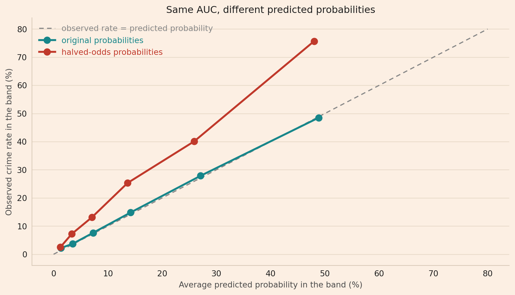
Halving every announcement’s odds of a crime leaves the AUC unchanged, while the probabilities then add up to about half the crimes that occur.

A model can rank outcomes well and still give probabilities far from how often the outcomes happen. Say a model gives each company announcement a probability of a market crime, here insider trading: somebody traded on the information before the announcement was public. The area under the receiver operating characteristic curve (AUC) measures such a model’s ranking: how often the model gives a higher probability to an announcement with a crime than to an announcement without a crime. Whether the probabilities agree with how often crimes happen is a separate property, called calibration, and the AUC does not measure calibration.

To show the difference, I take the logistic model from Logit and probit: what the coefficients mean and test it on 10,000 simulated announcements. Then I halve each announcement’s odds of a crime, the probability of a crime divided by the probability of no crime. Halving the odds keeps every announcement in the same order. The AUC stays at 0.747841, while the expected number of crimes, the sum of the predicted probabilities, decreases from 1,126 to 630, against 1,172 crimes observed.

Simulating the data

With real announcements I would not know which ones were crimes, because the records count an undetected crime as no crime. So I simulate 30,000 announcements, each with three variables: the size of the price move the announcement caused, how many people knew beforehand, and the size of the largest order placed before the announcement. Each variable is measured in standard deviations from its average, where a standard deviation measures how far values typically are from their average. A crime happens at random, with a probability that depends on the three variables through coefficients I set, the weights of the three variables. A logistic regression turns a weighted sum of the three variables into a probability between 0 and 1. I fit one to the first 20,000 announcements, the fitting sample, estimating its weights from them, and test it on the last 10,000, the test sample. The box below gives the formula and the code.

NoteHow the announcements are simulated

The true score of announcement \(i\) combines the three variables with the coefficients I set,

\[\eta_i = -2.4 + 1.1\,x_{1i} + 0.7\,x_{2i} - 0.5\,x_{3i}, \qquad x_{3i} = 0.8\,x_{1i} + 0.6\,u_i,\]

where \(x_1\), \(x_2\) and \(x_3\) are information_value, insiders_with_access and largest_order, and \(x_1\), \(x_2\) and \(u_i\) are independent draws from the standard normal distribution, which is bell-shaped with a mean of 0 and a standard deviation of 1, so \(x_3\) has a standard deviation of 1, since \(0.8^2 + 0.6^2 = 1\), and a correlation of 0.8 with \(x_1\), on a scale from −1 to 1 on which 1 would mean that the two move in perfect step. The block below turns each score into a probability of a crime with the logistic function, \(p_i = e^{\eta_i}/(1 + e^{\eta_i})\), which turns any score into a probability between 0 and 1: an announcement with all three variables at 0 has a score of \(-2.4\) and a probability of \(e^{-2.4}/(1 + e^{-2.4}) = 8.3\%\). The block then decides at random whether a crime happens, with that probability, independently across announcements.

import numpy as np
import pandas as pd

N_ANNOUNCEMENTS = 30000
N_FITTING = 20000                         # the other 10,000 are the test sample
rng = np.random.default_rng(11)           # fixed, so every number in the post reproduces

information_value = rng.normal(0, 1, N_ANNOUNCEMENTS)
insiders_with_access = rng.normal(0, 1, N_ANNOUNCEMENTS)
# 0.8 squared plus 0.6 squared is 1, so largest_order is drawn with a standard deviation of 1,
# like the other two variables, and a correlation of 0.8 with information_value.
largest_order = 0.8 * information_value + 0.6 * rng.normal(0, 1, N_ANNOUNCEMENTS)

variables = pd.DataFrame({"information_value": information_value,
                          "insiders_with_access": insiders_with_access,
                          "largest_order": largest_order})

# The coefficients I set, which I never give to a model below. Each one is a coefficient on
# the log odds, the logarithm of the probability of a crime divided by the probability of no
# crime.
TRUE_INTERCEPT = -2.4
TRUE_VARIABLE_COEFFICIENTS = {"information_value": 1.1, "insiders_with_access": 0.7,
                              "largest_order": -0.5}
VARIABLE_NAMES = list(TRUE_VARIABLE_COEFFICIENTS.keys())


def logistic_function(score):
    """Convert any score into a probability between 0 and 1.

    A score of 0 gives 0.50, a score of -4 gives about 0.02, and a score of 4 about 0.98.
    """
    return 1.0 / (1.0 + np.exp(-score))


# For each announcement, multiply each variable by its coefficient and add the three
# products, then pass that sum through the logistic function to get a probability.
true_coefficients = np.array(list(TRUE_VARIABLE_COEFFICIENTS.values()))
true_score = TRUE_INTERCEPT + variables.to_numpy() @ true_coefficients
true_probability = logistic_function(true_score)

# Draw each outcome: a crime whenever a random number between 0 and 1 is below the
# announcement's probability, which happens with exactly that probability.
crime_draw = rng.uniform(0, 1, N_ANNOUNCEMENTS)
is_crime = pd.Series((crime_draw < true_probability).astype(int))

# The first 20,000 announcements are the fitting sample and the last 10,000 the test sample.
# Every announcement is drawn the same way and independently of the others, so splitting by
# position is equivalent to a random split.
fitting_sample = np.arange(N_ANNOUNCEMENTS) < N_FITTING
test_sample = ~fitting_sample

# DataFrame.loc[rows, columns] selects rows and columns; omitting columns keeps all columns.
# Series.loc[rows] selects rows. Here, fitting_sample keeps the rows marked True.
print(f"announcements {N_ANNOUNCEMENTS:,}, crimes {is_crime.sum():,} ({is_crime.mean():.2%})")
print(f"  fitting sample {fitting_sample.sum():,}, crimes {is_crime.loc[fitting_sample].sum():,} "
      f"({is_crime.loc[fitting_sample].mean():.2%})")
print(f"  test sample    {test_sample.sum():,}, crimes {is_crime.loc[test_sample].sum():,} "
      f"({is_crime.loc[test_sample].mean():.2%})")
print(f"true probability ranges from {true_probability.min():.4f} to {true_probability.max():.4f}")
print(f"correlation between information_value and largest_order: "
      f"{np.corrcoef(information_value, largest_order)[0, 1]:.3f}")

announcements 30,000, crimes 3,425 (11.42%)
  fitting sample 20,000, crimes 2,253 (11.27%)
  test sample    10,000, crimes 1,172 (11.72%)
true probability ranges from 0.0017 to 0.8316
correlation between information_value and largest_order: 0.797

Of the 30,000 announcements, 3,425 are crimes, 11.4%: 2,253 in the fitting sample and 1,172 in the test sample. The true probabilities range from 0.0017 to 0.8316, and the correlation between information_value and largest_order is 0.797, close to the 0.8 that the formula sets.

The block below fits the logistic model with the statsmodels library, which gives each announcement a predicted probability of a crime.

import statsmodels.api as sm

# add_constant puts a column of ones in front of the three variables, and its coefficient is
# the intercept. disp=0 turns off the messages statsmodels prints while it searches for the coefficients.
design = sm.add_constant(variables)
logit = sm.Logit(is_crime.loc[fitting_sample], design.loc[fitting_sample]).fit(disp=0)

Testing ranking and calibration

I test the logistic model on the 10,000 announcements of the test sample in two ways.

Ranking concerns the order of the predicted probabilities. For a pair of announcements, one with a crime and one without, the model ranks the pair correctly when it gives the higher probability to the announcement with the crime. The AUC is the fraction of all such pairs that the model ranks correctly, counting a tie as half. Random ranking has an expected AUC of 0.5, and perfect ranking has an AUC of 1. An earlier post counts the AUC by hand.

Calibration concerns whether the predicted probabilities agree with how often crimes happen. Among 1,000 announcements given a probability of 10%, about 100 should turn out to be crimes, and the observed count can differ from 100 by chance.

To show what the AUC misses, I keep the announcements and their outcomes and change only the predicted probabilities: I halve each announcement’s odds and convert them back into probabilities, the halved-odds probabilities. A probability of 10% has odds of 0.10/0.90 = 0.111, which halve to 0.056, a probability of 0.056/(1 + 0.056) = 5.3%, and a probability of 50% becomes 33.3%. Higher odds always mean a higher probability, so every pair is ranked as before, and the AUC cannot change.

The expected number of crimes is the sum of the predicted probabilities. For example, 100 announcements at 5% should contain about 5 crimes. Comparing the expected number with the observed number of crimes checks calibration over the whole test sample.

from sklearn.metrics import roc_auc_score

test_design = design.loc[test_sample]
test_outcome = is_crime.loc[test_sample]

test_probability = logit.predict(test_design)
test_odds = test_probability / (1 - test_probability)
halved_odds = test_odds / 2                        # same order, half the odds
probability_from_halved_odds = halved_odds / (1 + halved_odds)

# The same announcements and the same outcomes, scored with two sets of probabilities.
auc_and_counts = pd.DataFrame({
    "AUC": [roc_auc_score(test_outcome, test_probability),
            roc_auc_score(test_outcome, probability_from_halved_odds)],
    "expected crimes": [test_probability.sum(), probability_from_halved_odds.sum()],
    "observed crimes": [test_outcome.sum(), test_outcome.sum()],
}, index=["original probabilities", "halved-odds probabilities"])
print(auc_and_counts.to_string(formatters={"AUC": "{:.6f}".format,
                                           "expected crimes": "{:,.0f}".format,
                                           "observed crimes": "{:,}".format}))

                               AUC expected crimes observed crimes
original probabilities    0.747841           1,126           1,172
halved-odds probabilities 0.747841             630           1,172

The AUC is 0.747841 for both sets of probabilities. The expected number of crimes decreases from 1,126 to 630, because every probability is lower. The observed number of crimes, 1,172, is the same in both rows, because the outcomes are unchanged. So a set of probabilities whose expected number of crimes is about half the observed number has the same AUC as the original set.

Checking calibration band by band

Comparing the expected number of crimes with the observed number is not enough, because probabilities that are too high for some groups of announcements and too low for others can cancel in the sum. So I sort the test announcements into six bands by predicted probability, from below 2% to above 40%, and compare each band’s average predicted probability with its observed crime rate, the share of its announcements that turn out to be crimes.

BAND_EDGES = [0, 0.02, 0.05, 0.10, 0.20, 0.40, 1.0]
BAND_NAMES = ["below 2%", "2% to 5%", "5% to 10%", "10% to 20%", "20% to 40%", "above 40%"]


def calibration_table(probability):
    """Compare the average predicted probability with the observed crime rate in each band.

    A band holding 700 announcements at an average predicted probability of 1.4% should
    contain about 10 crimes. The ratio column is the observed crime rate divided by the
    average predicted probability, so 1.00 is agreement.
    """
    # cut() assigns each predicted probability to a band, and the bands become the rows
    grouped = pd.DataFrame({"band": pd.cut(probability, BAND_EDGES, labels=BAND_NAMES,
                                           include_lowest=True),
                            "predicted": probability,
                            "crime": test_outcome})
    # observed=True keeps only the bands that hold announcements, because cut() makes a
    # category for every band whether or not it holds any announcements
    table = grouped.groupby("band", observed=True).agg(announcements=("crime", "size"),
                                                       predicted=("predicted", "mean"),
                                                       observed=("crime", "mean"))
    table["ratio"] = table["observed"] / table["predicted"]
    # the two probabilities in percent, like the prose
    table["predicted"] = 100 * table["predicted"]
    table["observed"] = 100 * table["observed"]
    table = table.rename(columns={"predicted": "predicted %", "observed": "observed %"})
    return table.round(2)


print("original probabilities:")
print(calibration_table(test_probability).to_string())
print("\nhalved-odds probabilities:")
print(calibration_table(probability_from_halved_odds).to_string())

original probabilities:
            announcements  predicted %  observed %  ratio
band                                                     
below 2%              719         1.37        2.23   1.62
2% to 5%             2297         3.50        3.70   1.06
5% to 10%            2889         7.28        7.62   1.05
10% to 20%           2594        14.16       14.80   1.05
20% to 40%           1266        27.10       27.88   1.03
above 40%             235        48.86       48.51   0.99

halved-odds probabilities:
            announcements  predicted %  observed %  ratio
band                                                     
below 2%             2218         1.25        2.52   2.01
2% to 5%             3475         3.35        7.22   2.16
5% to 10%            2506         7.09       13.17   1.86
10% to 20%           1355        13.63       25.31   1.86
20% to 40%            409        25.91       40.10   1.55
above 40%              37        48.01       75.68   1.58

Under the original probabilities, the band from 2% to 5% holds 2,297 announcements. Their average predicted probability is 3.50%, so they should contain about 80 crimes, because 2,297 × 3.50% = 80.4. The band contains 85 crimes, so its observed crime rate is 85/2,297 = 3.70%. The ratio column divides the observed crime rate by the average predicted probability, 3.70/3.50 = 1.06 here, so a ratio of 1 means that a band’s probabilities are right on average. The chart below plots each band as a point, with the average predicted probability on the horizontal axis and the observed crime rate on the vertical axis, so this band is the teal point at 3.50% across and 3.70% up.

import matplotlib.pyplot as plt

RED, TEAL, GREY = "#C0392B", "#17868A", "#888888"
# The site's chart colours: a cream background, a light grid and a pale frame, so every chart
# on the site has the same look.
BG, INK, GRID, SPINE, AXIS_TEXT = "#FCEFE3", "#1f1f1f", "#EADCCC", "#D5C6B4", "#4a4a4a"


def style_chart(figure, axis):
    """Give a finished chart the site's cream background, light grid and pale frame."""
    figure.patch.set_facecolor(BG)
    axis.set_facecolor(BG)
    axis.grid(True, axis="y", color=GRID, lw=1.0)
    axis.set_axisbelow(True)
    for side in ("top", "right"):
        axis.spines[side].set_visible(False)
    for side in ("left", "bottom"):
        axis.spines[side].set_color(SPINE)
    axis.tick_params(axis="both", length=0, colors=INK, pad=6)
    axis.xaxis.label.set_color(AXIS_TEXT)
    axis.yaxis.label.set_color(AXIS_TEXT)
    axis.title.set_color(INK)
    # each legend entry in the colour of its line
    legend = axis.get_legend()
    for text, line in zip(legend.get_texts(), legend.get_lines()):
        text.set_color(line.get_color())


# figsize is the figure's width and height in inches. "o-" draws each band as a point joined to
# the next by a line; lw is the line width and ms the size of the points. The grey dashed line,
# ls=(0, (4, 3)), marks where the observed rate equals the predicted probability.
figure, axis = plt.subplots(figsize=(9, 5.2))
axis.plot([0, 80], [0, 80], color=GREY, ls=(0, (4, 3)), lw=1.4,
          label="observed rate = predicted probability")
for name, probability, colour in [("original probabilities", test_probability, TEAL),
                                  ("halved-odds probabilities", probability_from_halved_odds, RED)]:
    band = calibration_table(probability)
    axis.plot(band["predicted %"], band["observed %"], "o-", color=colour, lw=2.4, ms=8,
              label=name)

axis.set_xlabel("Average predicted probability in the band (%)")
axis.set_ylabel("Observed crime rate in the band (%)")
axis.set_title("Same AUC, different predicted probabilities")
axis.legend(frameon=False)
style_chart(figure, axis)
plt.tight_layout()
plt.savefig("calibration_bands.png", dpi=140, bbox_inches="tight", facecolor=BG)
plt.show()

The grey dashed line marks where the observed crime rate equals the average predicted probability. The teal points, for the original probabilities, are almost on the line, with ratios of 0.99 to 1.06 except 1.62 in the band below 2%. All six red points, for the halved-odds probabilities, are above the line, with ratios of 1.55 to 2.16, so in every band the observed crime rate is well above the average halved-odds probability. Halving the odds also moves announcements into lower bands, so a red point and a teal point in the same band hold different announcements.

Observed crime rates vary by chance, so even a calibrated model does not put every point exactly on the grey dashed line. Whether a gap such as 16 crimes against about 10 expected in the band below 2% shows that the model is not calibrated depends on the size of the gap and on how much a count that small varies by chance.

Limitations

The simulation supplies the outcome. With real records, the outcome would come from suspicious transaction reports, which cover only what somebody filed, or from prosecutions, which cover only what reached a court. Another post models crimes when some outcomes are unobserved.

The split assumes independent announcements. Taking the first 20,000 and the last 10,000 is equivalent to a random split only because I draw every announcement the same way. With real records, a split by date would also test the model on a later period.

The data come from the logistic model. With real data, the logistic model is not known to have generated the outcomes, so a real model’s probabilities can be less well calibrated than here.

The threshold is a separate decision. Acting on a probability needs a threshold that weighs the cost of missing a crime against the cost of investigating trading that involved no crime. Neither the AUC nor calibration sets the threshold.

Conclusion

Halving the odds does not change the AUC, because the AUC measures only ranking. The takeaway is that a model’s probabilities need their own calibration check, band by band, on announcements the model was not fitted to.

Read next

• Logit and probit: what the coefficients mean The model tested here, and how to read its coefficients as changes in the probability of a crime.
• Two models with 99% accuracy can rank an offender differently Where the AUC comes from, counted by hand on 100 traders.
• How to validate a daily loss forecast The same problem for a loss forecast: exceeded on 5% of all days and wrong on both calm and volatile days.

Disclaimer: a teaching example on simulated data. I choose the coefficients and generate the outcomes. Not investment advice.