How constant are discount rates?
How constant are discount rates? When I learned the DCF model as an undergraduate, I was taught to compute a discount rate once and apply it to every year of projected cash flows. That treats the rate as constant, even though its components all move over time. A firm’s cost of capital holds its relative standing for a year or two, then drifts over five. Bali, Engle and Murray (2016) measure persistence as the cross-sectional correlation between a firm’s characteristic at one date and its value some months later, averaged over every starting date. I test whether the weighted average cost of capital (WACC) and its two main components, the cost of equity and the cost of debt, stay that persistent across US firms.
They do not, past the first year or two. WACC correlates 0.7 with its own value one year later. At five years the correlation is 0.2. Cost of debt holds up best over the long horizon, and cost of equity fades fastest.
Persistence here is one number. It is the correlation between a firm’s value today and its value some years later, across all firms. A correlation near one means firms keep their order. A correlation near zero means the order reshuffles.
The variables
- WACC: the blended cost of capital LSEG StarMine reports for each firm, with equity and debt weighted by their share of the capital structure.
- Cost of equity: the equity component, from a CAPM-style estimate with a rolling beta.
- Cost of debt: the after-tax cost of debt component.
Starting point
The analysis runs off one long-format panel of month-end WACC values. Building it is a separate job that depends on the data vendor. I pull the StarMine cost-of-capital fields from LSEG Workspace. Because the data is licensed, the raw file stays off this page, and I show the code without running it here. The panel covers up to 6,076 US firms across 125 month-end dates, from December 2015 to April 2026.
Step 1. Persistence
For each lag I take the cross-section of a variable at month t and the cross-section at month t + tau, keep the firms present in both, winsorize each period at 0.5% to cap outliers, and correlate them. Then I average that correlation over every starting month. I do this at lags of 12, 24, 36, 48, and 60 months, which are one through five years.
PERSIST_LAGS = [12, 24, 36, 48, 60]           # lags in months: 1 to 5 years
WINS_Q       = 0.005                           # winsorize each tail at 0.5%
MIN_FIRMS    = 30                              # skip months with too few firms

def winsorize(s, q=WINS_Q):
    lo, hi = s.quantile(q), s.quantile(1 - q)  # within-period cutoffs
    return s.clip(lo, hi)                       # cap both tails, drop nothing

def persistence(panel, lags=PERSIST_LAGS):
    """Average cross-sectional correlation of a variable at t and t+tau."""
    dates, out = panel.index, {}
    for tau in lags:
        rhos = []
        for i in range(len(dates) - tau):      # every starting month t
            a = panel.iloc[i].dropna()          # the cross-section at t
            b = panel.iloc[i + tau].dropna()    # the cross-section at t+tau
            common = a.index.intersection(b.index)   # firms present in both
            if len(common) < MIN_FIRMS:         # too few pairs for a correlation
                continue
            a, b = winsorize(a[common]), winsorize(b[common])
            rhos.append(a.corr(b))              # Pearson correlation across firms
        out[tau] = np.mean(rhos)                # average over all starting months
    return out
The winsorizing protects the correlation from a handful of extreme values, such as a bankruptcy-driven cost of equity, without dropping any firm. Lesson 19 covers the rolling-window mechanics behind the panel.
Step 2. The persistence table
I run the same measure on each of the three variables and collect one row each. Each column is the average correlation at that horizon.
FIELDS = {
    'TR.WACC':             'WACC',
    'TR.WACCCostofEquity': 'Cost of Equity',
    'TR.WACCCostofDebt':   'Cost of Debt',
}

rows = []
for field, name in FIELDS.items():
    panel = (long_df[long_df['field'] == field]           # one variable
             .pivot_table(index='date', columns='ric', values='value')
             .sort_index()
             .resample('ME').last())                       # common month-end grid
    rho = persistence(panel)                               # {tau: average correlation}
    rows.append({'variable': name,
                 **{f'{t // 12}y': rho[t] for t in PERSIST_LAGS}})

table = pd.DataFrame(rows).set_index('variable')
print(table.round(3).to_string())
1y 2y 3y 4y 5y
variable
WACC 0.668 0.523 0.403 0.305 0.229
Cost of Equity 0.774 0.630 0.490 0.363 0.249
Cost of Debt 0.644 0.534 0.467 0.438 0.403A firm’s WACC correlates 0.7 with its own value one year later. At two years the correlation is 0.5, at three years 0.4, and by five years 0.2. So, a firm that stands high on cost of capital today has only a weak tendency to still stand high five years on.
Cost of equity is the most persistent of the three at one year, at 0.8, and decays to 0.2 at five years. It starts highest and decays the fastest.
Cost of debt starts lower, at 0.6 one year out, and holds its standing longer. At five years it is still 0.4, the highest of the three at that horizon.
Results
fig, ax = plt.subplots(figsize=(10, 6))
for name in table.index:                          # one line per variable
    ax.plot([1, 2, 3, 4, 5], table.loc[name], marker='o', lw=2, label=name)

ax.set_xlabel('Years ahead')
ax.set_ylabel('Correlation with today')
ax.set_title('How constant are discount rates?')
ax.set_ylim(0, 1); ax.set_xticks([1, 2, 3, 4, 5])
ax.legend(loc='lower left', frameon=True); ax.grid(alpha=0.3)
plt.tight_layout(); plt.savefig('wacc_persistence_decay.png', dpi=150); plt.show()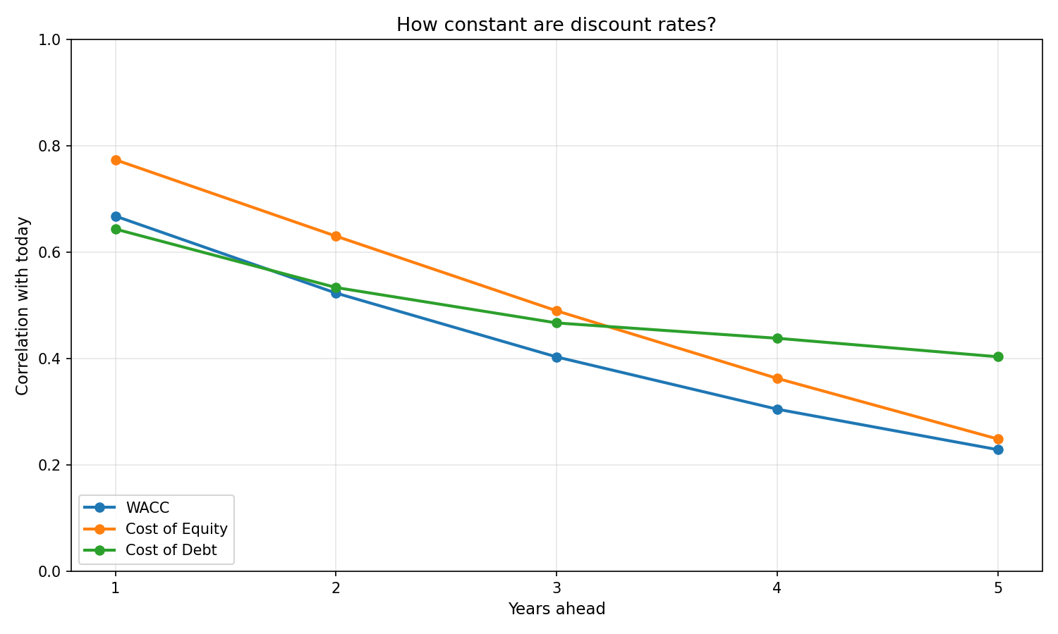
All three lines start below 0.8 and slope down. WACC and cost of equity fall together toward 0.2 by year five. Cost of debt flattens out and stays near 0.4.
What this does not settle
Mechanical overlap. LSEG computes WACC with a beta estimated over a rolling window of about 60 months. Two cross sections less than five years apart therefore share some of the same beta input, so the one-year and two-year correlations read higher than the firms’ true persistence. The five-year column is the cleanest of the five.
One vendor’s definition. The numbers describe LSEG’s WACC and its components. I use the vendor’s figures and do not compute a WACC myself. A different beta window, tax rate, or capital-weight rule would move the levels and could move the persistence.
Overlapping windows. The correlation at each lag averages over every starting month, and windows one month apart share almost all of their firms. The 125 months are not 125 independent draws, so I do not attach a confidence interval to any figure.
A short panel. The sample is 125 months, from December 2015 to April 2026. The five-year correlation rests on the 65 starting months that have a partner 60 months later. A longer history would pin the tail down better.
What it means
Across US firms, a firm’s cost of capital holds its relative standing for a year or two and then drifts. WACC correlates 0.7 with itself one year out and 0.2 at five years. Cost of debt is the stickiest of the three components at long horizons, and WACC the least sticky. A firm’s current WACC standing is a fair guide to next year and a weak guide to five years out. So, a single WACC applied across a multi-year DCF is a modelling convenience, and it does not claim that discount rates hold constant. The takeaway is that a firm’s cost of capital is only moderately persistent, because its standing fades most of the way to noise within five years.
Read next
- The Magic Formula worked. Just not lately. Cheapness and return on capital, the levers a discount rate is meant to price.
- Avoiding bad companies matters as much as finding great ones Profitability and quality, measured the same point-in-time way.
Disclaimer: this is a descriptive statistical analysis for discussion purposes only. Not investment advice.
Data: WACC and its components for US firms from LSEG StarMine, accessed through Workspace (licensed). I do not reproduce the raw file here.