How to test whether a characteristic predicts future returns

Python
Statistics
Backtesting
Code
A portfolio sort and a Fama-MacBeth regression on the same simulated data both report that the characteristic predicts returns. The sort gives a difference of 0.822% a month between the extreme groups. The regression gives a slope of 0.2293% a month per standard deviation.
Published

September 5, 2026

Source: Image by author using ChatGPT

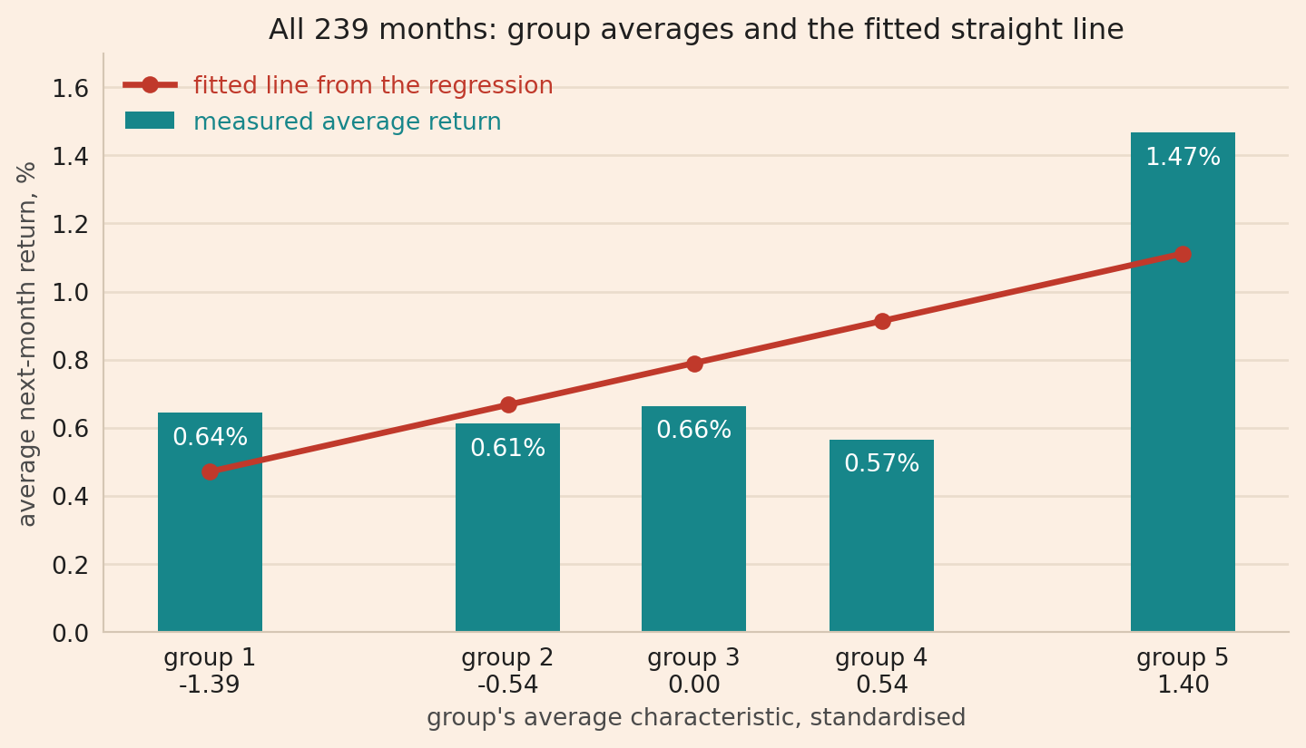
A portfolio sort and a linear Fama-MacBeth regression can both report that a characteristic predicts returns while describing the relation very differently. When only the top fifth of stocks receives extra expected return, average return is close to 0.6% a month across the first four groups and 1.47% in the fifth. The fitted regression instead predicts an increase of 0.12 to 0.20 percentage points between every pair of adjacent groups.

A characteristic is one number attached to a stock at a point in time: its size, its book-to-market ratio, its return over the past year. A portfolio sort ranks stocks on it each month, splits them into five groups, and compares the returns of those groups over the month after. A Fama-MacBeth regression estimates a slope on the characteristic each month and averages the slopes.

The two methods assume different things. A portfolio sort is nonparametric, so it imposes no functional form on the relation between the characteristic and the return. The Fama-MacBeth regression used here imposes a linear relation.

In this post, I run both methods on data I simulate myself, so the true relation is known in advance and each method can be judged against it. When expected return changes linearly with the characteristic, the two methods describe the same pattern. So I simulate two markets. In the first, one standard deviation more of the characteristic adds 0.24 percentage points to next month’s expected return, the same amount at every level. In the second, only the top fifth of stocks receives extra expected return.

The market I simulate

The market holds 500 stocks over 240 months. Every stock has a characteristic that changes gradually from month to month. I standardise it across stocks each month so that a value of 1 always means the same thing, one standard deviation above the average stock.

Next month’s return has two parts. The first is the expected return: 0.6%, plus 0.24 percentage points for every standard deviation of this month’s characteristic. The second is the stock’s own noise, drawn fresh each month with a standard deviation of 12%. Every return here is measured above cash.

import numpy as np
import pandas as pd

STOCKS = 500                        # how many stocks the market holds
MONTHS = 240                        # twenty years of monthly observations
CHARACTERISTIC_PERSISTENCE = 0.95   # how much of last month's value persists into this month
FIRM_NOISE = 0.12                   # standard deviation of one stock's own monthly return
AVERAGE_EXCESS_RETURN = 0.006       # the average stock's return above cash in a month
RETURN_PER_SD = 0.0024              # extra expected return from one standard deviation
CORRELATION_WITH_RETURN = 0.8       # correlation with the return characteristic, not with returns
GROUPS = 5                          # how many portfolios the sort forms

RED, BLUE, GREY = "#C44E52", "#1F77B4", "#BBBBBB"


def standardise(values):
    """Rescale each month to average 0 and standard deviation 1.

    One row is one month. Doing this month by month fixes what a value of 1 means
    without touching how the stocks are ranked against each other inside that month.
    """
    standardised = np.empty_like(values)
    for month in range(len(values)):
        this_month = values[month]
        standardised[month] = (this_month - this_month.mean()) / this_month.std(ddof=1)
    return standardised


def slow_moving_characteristic(generator, months, stocks):
    """One number per stock per month that mostly persists from the month before.

    A real characteristic changes slowly. A firm's book-to-market ratio this month is
    close to last month's, so the loop keeps 95% of the previous value and adds fresh
    noise on top. The square root sizes that noise so the series keeps a standard
    deviation of one instead of growing over the sample.
    """
    fresh_share = np.sqrt(1 - CHARACTERISTIC_PERSISTENCE ** 2)
    values = np.empty((months, stocks))
    values[0] = generator.normal(0, 1, stocks)
    for month in range(1, months):
        carried_over = CHARACTERISTIC_PERSISTENCE * values[month - 1]
        values[month] = carried_over + fresh_share * generator.normal(0, 1, stocks)
    return standardise(values)

I simulate three characteristics. The return characteristic affects next month’s expected return. The unrelated characteristic does not. The correlated characteristic is correlated with the return characteristic but has no direct effect on returns.

def simulate_market(seed):
    """Build one market and return it as a table with one row per stock per month."""
    generator = np.random.default_rng(seed)

    characteristic = slow_moving_characteristic(generator, MONTHS, STOCKS)
    unrelated = slow_moving_characteristic(generator, MONTHS, STOCKS)
    independent_component = slow_moving_characteristic(generator, MONTHS, STOCKS)

    # The correlated characteristic combines 0.8 times the return characteristic with an
    # independent component. The square-root term keeps the variance at one before
    # standardisation.
    correlated_characteristic = standardise(
        CORRELATION_WITH_RETURN * characteristic
        + np.sqrt(1 - CORRELATION_WITH_RETURN ** 2) * independent_component)

    # Each stock's own return component, drawn separately for every stock and month
    firm_specific = generator.normal(0, FIRM_NOISE, (MONTHS, STOCKS))

    stock_return = AVERAGE_EXCESS_RETURN + firm_specific
    # Row 1 onward gets the characteristic from the row above, so this month's return
    # uses last month's characteristic and never its own.
    stock_return[1:] += RETURN_PER_SD * characteristic[:-1]

    # repeat gives 0,0,0,...,1,1,1,... and tile gives 0,1,2,...,0,1,2,..., so the two
    # columns together name every stock in every month exactly once. ravel lays each
    # months-by-stocks table out in that same order.
    panel = pd.DataFrame({
        "month": np.repeat(np.arange(MONTHS), STOCKS),
        "stock": np.tile(np.arange(STOCKS), MONTHS),
        "characteristic": characteristic.ravel(),
        "unrelated": unrelated.ravel(),
        "correlated": correlated_characteristic.ravel(),
        "stock_return": stock_return.ravel(),
    })

    # shift moves values by position rather than by date, so the rows must be ordered
    # by month within each stock before it is used.
    panel = panel.sort_values(["stock", "month"]).reset_index(drop=True)
    panel["next_return"] = panel.groupby("stock")["stock_return"].shift(-1)
    return panel


# One fixed seed, so the page draws the same market every time it is rendered.
panel = simulate_market(0)

# The last month of every stock has no next month, so it cannot be used.
traded = panel.dropna(subset=["next_return"]).copy()

print(panel.head(3).to_string(index=False))
print(f"\n{len(panel):,} rows, {panel.month.nunique()} months, {panel.stock.nunique()} stocks")
 month  stock  characteristic  unrelated  correlated  stock_return  next_return
     0      0        0.150422   1.491289   -0.455074     -0.178966    -0.186188
     1      0        0.565223   1.612921   -0.082753     -0.186188    -0.040452
     2      0        0.883030   1.420783    0.107979     -0.040452    -0.298372

120,000 rows, 240 months, 500 stocks

The next_return column is what makes this a prediction. The characteristic on a row is measured at the end of that month, and the return beside it comes from the month after. No information from next month enters the characteristic used to form the groups.

One stock at a time

I generated the returns, so I know that one standard deviation more of the characteristic adds 0.24 percentage points to expected return. The question is whether that is visible in the data. Every stock is plotted against its return over the month after, first for a single month and then for all 239 of them.

import matplotlib.pyplot as plt

one_month = traded[traded.month == 100]
characteristic_axis = np.array([-3.2, 3.2])   # two x-values are enough to draw a straight line
expected_return_at_axis = (AVERAGE_EXCESS_RETURN + RETURN_PER_SD * characteristic_axis) * 100

fig, axes = plt.subplots(1, 2, figsize=(10, 4.2))

axes[0].scatter(one_month["characteristic"], one_month["next_return"] * 100,
                s=5, alpha=0.55, color=BLUE, linewidths=0)
axes[0].plot(characteristic_axis, expected_return_at_axis, color=RED, lw=2)
axes[0].set_title("one month, 500 stocks")
axes[0].set_ylabel("next month's return, %")

axes[1].scatter(traded["characteristic"], traded["next_return"] * 100,
                s=5, alpha=0.10, color=BLUE, linewidths=0)
axes[1].plot(characteristic_axis, expected_return_at_axis, color=RED, lw=2)
axes[1].set_title("all 239 months, 119,500 observations")

for axis in axes:
    axis.set_xlabel("characteristic at the end of the month")
    axis.set_ylim(-45, 45)

plt.tight_layout()
plt.savefig("ps_one_stock.png", dpi=140, bbox_inches="tight")
plt.show()

def characteristic_return_correlation(block):
    """The correlation between the characteristic and the next return, inside one month."""
    return block["characteristic"].corr(block["next_return"])


# Running it inside a groupby keeps each month separate, which is how every method in
# this post works: one cross-section at a time, then an average over the months.
monthly_correlation = (traded.groupby("month")[["characteristic", "next_return"]]
                             .apply(characteristic_return_correlation))

monthly_standard_deviation = traded.next_return.std(ddof=1) * 100
print(f"one stock's monthly return, standard deviation: {monthly_standard_deviation:.2f}%")
print(f"average cross-sectional correlation:            {monthly_correlation.mean():.4f}")

# The widest difference the simulation puts between two stocks in the same month
range_by_month = traded.groupby("month")["characteristic"].agg(["min", "max"])
widest_difference = (RETURN_PER_SD * (range_by_month["max"] - range_by_month["min"])).mean()
print(f"lowest to highest stock, expected return:      {widest_difference * 100:.2f} pp")
# Square each month's correlation and then average, rather than squaring the average. The
# two are not the same number, and this one is the share of variation explained.
print(f"average monthly r-squared:                      {(monthly_correlation ** 2).mean():.5f}")
one stock's monthly return, standard deviation: 12.02%
average cross-sectional correlation:            0.0205
lowest to highest stock, expected return:      1.41 pp
average monthly r-squared:                      0.00256

The red line is the expected return implied by the simulation. The correlation between the characteristic and the next return averages 0.02 across months, and the average monthly r-squared is 0.0026, so the characteristic accounts for about a quarter of one percent of the variation in next month’s return. A stock’s own noise has a standard deviation of 12% a month, and expected return differs by 1.41 percentage points between the lowest and the highest stock in an average month. The stock-level scatter therefore gives almost no visual indication of the relation, on data generated to contain it.

Five groups

I follow the portfolio-sort procedure in Bali, Engle and Murray’s Empirical Asset Pricing: The Cross Section of Stock Returns. It has four steps: calculate the breakpoints, form the portfolios, average the return inside each portfolio in each month, then compare those averages across portfolios. The breakpoints are percentiles of that month’s cross-section, and for five portfolios they are the 20th, 40th, 60th and 80th.

pd.qcut does exactly that: it takes one month’s values and returns which fifth each stock belongs to.

def five_groups(month_values):
    """Label one month's stocks 0 to 4 by which fifth of the sorted range they belong to."""
    return pd.qcut(month_values, GROUPS, labels=False)


def sort_into_groups(frame, column):
    """Give every row a group number from 1 to 5, from its rank within its own month.

    transform runs five_groups inside each month and hands the labels back in the
    original row order, so the breakpoints belong to the month rather than to the
    whole sample. That is what the method requires.
    """
    return frame.groupby("month")[column].transform(five_groups) + 1   # qcut labels from 0


def group_returns(frame, column):
    """Average next-month return of each group. One row per month, one column per group."""
    work = frame.copy()
    work["group"] = sort_into_groups(work, column)
    # unstack turns the group label into columns, so each row becomes one month
    return work.groupby(["month", "group"])["next_return"].mean().unstack()


by_group = group_returns(traded, "characteristic")

# assign adds a column and hands back a new table, leaving traded as it was
holdings = traded.assign(group=sort_into_groups(traded, "characteristic"))

print("stocks in each group each month:", holdings.groupby(["month", "group"]).size().unique())
print("\naverage return, % a month")
for group in by_group.columns:
    print(f"  group {group}: {by_group[group].mean() * 100:.3f}")
stocks in each group each month: [100]

average return, % a month
  group 1: 0.258
  group 2: 0.575
  group 3: 0.634
  group 4: 0.673
  group 5: 1.018

Every stock is weighted the same inside its group. Value weighting uses market capitalisation instead, and is generally taken to be closer to what an investor could have realised, because it puts the money in the large and liquid names. The simulation has no market-capitalisation variable, so I use equal weights.

The expected returns implied by the simulation can be drawn on the same axes. A group’s expected return is 0.6% plus 0.24 percentage points times its average characteristic, and that average follows from the normal distribution the characteristic was drawn from.

from scipy.stats import norm

# The average of a standard normal above its 80th percentile. This is the expected
# average characteristic of the top fifth, and the bottom fifth is its mirror image.
top_fifth_expected = norm.pdf(norm.ppf(0.8)) / 0.2
expected_difference_year = RETURN_PER_SD * 2 * top_fifth_expected * 1200

average_characteristic = holdings.groupby("group")["characteristic"].mean()

print(f"the normal distribution implies      {top_fifth_expected:+.3f}")
print(f"this market's top fifth averages     {average_characteristic[GROUPS]:+.3f}")
print(f"this market's bottom fifth averages  {average_characteristic[1]:+.3f}")
print(f"\nexpected top-minus-bottom difference: {expected_difference_year:.2f}% a year "
      f"between the extreme groups")
the normal distribution implies      +1.400
this market's top fifth averages     +1.398
this market's bottom fifth averages  -1.404

expected top-minus-bottom difference: 8.06% a year between the extreme groups
expected_return_by_group = (AVERAGE_EXCESS_RETURN + RETURN_PER_SD * average_characteristic) * 100

fig, axis = plt.subplots(figsize=(7.6, 4.2))
axis.bar(by_group.columns, by_group.mean() * 100, color=BLUE, width=0.62, label="what the sort found")
axis.plot(by_group.columns, expected_return_by_group, "o", color=RED, ms=8,
          label="what the simulation implies")
axis.set_xlabel("group, sorted low to high on the characteristic")
axis.set_ylabel("average return, % a month")
axis.set_title("Average return of each group of 100 stocks")
axis.legend(frameon=False)

plt.tight_layout()
plt.savefig("ps_five_groups.png", dpi=140, bbox_inches="tight")
plt.show()

Average return is 0.26% a month in the lowest group and 1.02% in the highest. The red dots are the expected returns implied by the simulation, and the bars match them. Nothing in the sorting code uses the 0.24, the return equation or the seed. It ranks stocks on a number and averages what happened next.

The middle groups are not perfectly ordered. Groups 3 and 4 are closer together than the simulation implies, because each group average has its own sampling error. A monotonic pattern across the groups is supporting evidence. For this example, where expected return increases with the characteristic, I summarise the sort with the difference between the ends.

Why grouping works

Take n stocks from the top fifth and n from the bottom fifth, and increase n.

def difference_at_group_size(frame, size):
    """Top-minus-bottom return each month, holding `size` stocks drawn from the end fifths.

    The two fifths are the same whatever `size` is, so only the averaging changes. Taking
    the `size` most extreme stocks instead would also change how extreme the characteristic
    is, and the expected difference would vary with it.
    """
    stocks_in_a_fifth = len(frame["stock"].unique()) // GROUPS
    monthly = []
    for month, block in frame.groupby("month"):
        ordered = block.sort_values("characteristic")
        bottom_fifth = ordered.head(stocks_in_a_fifth)
        top_fifth = ordered.tail(stocks_in_a_fifth)
        # random_state=month keeps the draw the same every time the page is built
        bottom = bottom_fifth.sample(size, random_state=month)["next_return"].mean()
        top = top_fifth.sample(size, random_state=month)["next_return"].mean()
        monthly.append(top - bottom)
    return pd.Series(monthly)


expected_difference = RETURN_PER_SD * 2 * top_fifth_expected

group_size_rows = []
for size in (1, 10, 50, 100):
    difference = difference_at_group_size(traded, size)
    noise = difference.std(ddof=1)
    group_size_rows.append({"stocks a side": size,
                            "expected difference %": expected_difference * 100,
                            "month-to-month noise %": noise * 100,
                            "difference over noise": expected_difference / noise})

print(pd.DataFrame(group_size_rows).round(3).to_string(index=False))
 stocks a side  expected difference %  month-to-month noise %  difference over noise
             1                  0.672                  16.189                  0.042
            10                  0.672                   5.609                  0.120
            50                  0.672                   2.270                  0.296
           100                  0.672                   1.679                  0.400

Both sides always draw from the same two fifths, so the expected difference is 0.67% a month at every group size. Only the averaging changes: the month-to-month standard deviation of the difference is 16.2% with one stock a side and 1.7% with a hundred.

Taking the single most extreme stock a side instead would make the expected difference 1.41% a month, because that stock has far more of the characteristic than the average stock in its fifth.

Firm-specific returns are drawn separately for every stock, so averaging a hundred of them divides their standard deviation by roughly ten. The expected return from the characteristic does not average away, because every stock in the group has a similar amount of the characteristic. Averaging therefore reduces the noise and preserves the expected difference, even though that difference is difficult to see in the stock-level scatter.

The long-short portfolio

In trading terms the top-minus-bottom difference is a long-short position: hold the top group, sell the bottom group short, and the difference is the return on that position.

difference = by_group[GROUPS] - by_group[1]


def describe(monthly_return):
    """Average, annual figures and a t-statistic for one series of monthly returns."""
    average = monthly_return.mean()
    deviation = monthly_return.std(ddof=1)      # ddof=1 is the sample formula
    months = len(monthly_return)
    return {
        "% a month": average * 100,
        "% a year": average * 1200,                       # twelve months, without compounding
        "volatility, % a year": deviation * np.sqrt(12) * 100,
        "Sharpe ratio": average / deviation * np.sqrt(12),
        "t-statistic": average / (deviation / np.sqrt(months)),
    }


for name, value in describe(difference).items():
    print(f"{name:>22}: {value:8.2f}")
print(f"{'months':>22}: {len(difference):8d}")
             % a month:     0.76
              % a year:     9.12
  volatility, % a year:     5.82
          Sharpe ratio:     1.57
           t-statistic:     7.00
                months:      239

A t-statistic of 7.0 means the average of these 239 monthly returns is seven standard errors from zero. A 5% test uses a threshold near 2.0. Harvey, Liu and Zhu (2016) argue that 2.0 is too low once many characteristics have been tested.

The 239 monthly returns form a time series, and an autocorrelated series makes the plain standard error wrong in either direction. Newey and West (1987) correct for that. I use six lags for these monthly returns.

def newey_west_t(monthly_return, lags=6):
    """t-statistic on the average, with Newey and West (1987) standard errors.

    The plain standard error assumes each month is independent of the last. This one
    also adds in how correlated months `lag` apart are, each term weighted down as the
    distance grows. Only the denominator changes, so the average itself is untouched.
    """
    values = np.asarray(monthly_return, dtype=float)
    months = len(values)
    deviations = values - values.mean()

    variance = (deviations * deviations).sum() / months
    for lag in range(1, lags + 1):
        weight = 1 - lag / (lags + 1)
        # each month lined up against the month `lag` later
        together = (deviations[lag:] * deviations[:-lag]).sum() / months
        variance += 2 * weight * together

    return values.mean() / np.sqrt(variance / months)


print(f"plain t-statistic:       {describe(difference)['t-statistic']:.2f}")
print(f"Newey-West t-statistic:  {newey_west_t(difference):.2f}")

# How correlated these monthly differences are, which is what the correction
# is for. Each month lined up against the one before it, scaled to range from -1 to 1.
deviations = difference - difference.mean()
month_on_month = (deviations[1:].values * deviations[:-1].values).sum() / (deviations ** 2).sum()
print(f"first-order autocorrelation: {month_on_month:.2f}"
      f"   (one standard error is {1 / np.sqrt(len(difference)):.2f})")


def sorted_portfolio_table(by_group, label):
    """One printed row of annual returns and one of t-statistics, as the journals show it.

    Bali, Engle and Murray present a univariate sort as the average excess return of each
    portfolio with its Newey-West t-statistic in brackets underneath, and the difference
    in the last column. They drop the standard error and the p-value because the
    t-statistic already contains the same information.
    """
    difference = by_group[GROUPS] - by_group[1]
    portfolios = list(by_group.columns) + [f"{GROUPS}-1"]
    series = [by_group[group] for group in by_group.columns] + [difference]

    header = "".join(f"{str(name):>9}" for name in portfolios)
    returns = "".join(f"{one.mean() * 1200:>9.2f}" for one in series)
    t_values = "".join(f"{'(' + format(newey_west_t(one), '.2f') + ')':>9}" for one in series)

    print(f"{label}\n{'':>16}{header}\n{'return, % a year':>16}{returns}\n{'':>16}{t_values}")


sorted_portfolio_table(by_group, "\nsorted on the characteristic")
plain t-statistic:       7.00
Newey-West t-statistic:  5.66
first-order autocorrelation: 0.08   (one standard error is 0.06)

sorted on the characteristic
                        1        2        3        4        5      5-1
return, % a year     3.10     6.90     7.61     8.08    12.21     9.12
                   (2.85)   (7.15)   (8.71)   (9.07)  (12.59)   (5.66)

The correction takes the t-statistic from 7.0 to 5.7. The firm-specific part of each return was drawn fresh every month, so the noise is independent from one month to the next. The characteristic is persistent, so the expected difference varies slightly across months, but the variation is small relative to the noise. In this sample the first-order autocorrelation is 0.08 with an approximate standard error of 0.06, so there is little evidence of serial correlation. “I report the Newey-West t-statistic anyway. For real sorted portfolios, whose returns can be autocorrelated, the size of the correction depends on the return series and the number of lags.”

A characteristic with no effect

The unrelated characteristic is generated the same way as the return characteristic and appears in no return equation. I run the identical four steps on it.

unrelated_groups = group_returns(traded, "unrelated")
unrelated_difference = unrelated_groups[GROUPS] - unrelated_groups[1]

print("average return, % a month, by group")
print("  characteristic:     ", (by_group.mean() * 100).round(3).to_list())
print("  unrelated:          ", (unrelated_groups.mean() * 100).round(3).to_list())
print(f"\nunrelated, top minus bottom: {unrelated_difference.mean() * 1200:.2f}% a year, "
      f"t {describe(unrelated_difference)['t-statistic']:.2f}, "
      f"Newey-West t {newey_west_t(unrelated_difference):.2f}")
average return, % a month, by group
  characteristic:      [0.258, 0.575, 0.634, 0.673, 1.018]
  unrelated:           [0.566, 0.693, 0.686, 0.503, 0.71]

unrelated, top minus bottom: 1.73% a year, t 1.26, Newey-West t 1.19
fig, axes = plt.subplots(1, 2, figsize=(10, 4.0), sharey=True)

axes[0].bar(by_group.columns, by_group.mean() * 100, color=BLUE, width=0.62)
axes[0].set_title("sorted on the characteristic")
axes[0].set_ylabel("average return, % a month")

axes[1].bar(unrelated_groups.columns, unrelated_groups.mean() * 100, color=GREY, width=0.62)
axes[1].set_title("sorted on the unrelated characteristic")

for axis in axes:
    axis.axhline(AVERAGE_EXCESS_RETURN * 100, color=RED, lw=1.4)   # the average stock's return
    axis.set_xlabel("group, low to high")

plt.tight_layout()
plt.savefig("ps_null.png", dpi=140, bbox_inches="tight")
plt.show()

Average returns are 0.57, 0.69, 0.69, 0.50 and 0.71% a month. They are close to the red line, which is the average stock’s return, and they do not increase across the groups. The difference between the ends is 1.73% a year with a t-statistic of 1.26, below the usual threshold of 2.0.

Even though the unrelated characteristic has no effect on returns, this twenty-year sample produces a 1.73% annual top-minus-bottom difference. One sample cannot show how often sampling noise produces a difference of that size, so I simulate 1,000 markets.

A thousand markets

With real data we observe one sample. In a simulation I can repeat the same experiment 1,000 times, once with the extra expected return in place and once without it.

def sorted_group_means(characteristic, stock_return):
    """Average next-month return of each equal-sized group, on plain arrays.

    Same answer as group_returns above. This version has to run thousands of times, so
    it skips pandas: argsort puts each month's stocks in order of the characteristic,
    take_along_axis reorders that month's returns to match, and reshape cuts each
    ordered row into GROUPS blocks of equal size.
    """
    order = np.argsort(characteristic[:-1], axis=1, kind="stable")
    ranked = np.take_along_axis(stock_return[1:], order, axis=1)
    return ranked.reshape(ranked.shape[0], GROUPS, -1).mean(axis=2)


def one_market_difference(seed, return_per_sd, months=MONTHS, stocks=STOCKS):
    """Build one market and return its top-minus-bottom result: % a year, and a t."""
    generator = np.random.default_rng(seed)
    characteristic = slow_moving_characteristic(generator, months, stocks)
    stock_return = AVERAGE_EXCESS_RETURN + generator.normal(0, FIRM_NOISE, (months, stocks))
    stock_return[1:] += return_per_sd * characteristic[:-1]

    group_means = sorted_group_means(characteristic, stock_return)
    difference = group_means[:, -1] - group_means[:, 0]
    standard_error = difference.std(ddof=1) / np.sqrt(len(difference))
    return difference.mean() * 1200, difference.mean() / standard_error


results = {}
for label, return_per_sd in (("with extra expected return", RETURN_PER_SD), ("with no extra expected return", 0.0)):
    # Start with an empty list, work through the seeds, collect one market's result each
    outcomes = []
    for market_number in range(1000):
        difference_percent, t_statistic = one_market_difference(
            10_000 + market_number, return_per_sd)
        outcomes.append({"difference": difference_percent, "t": t_statistic})
    results[label] = pd.DataFrame(outcomes)

print(f"expected top-minus-bottom difference: {expected_difference_year:.2f}% a year\n")
for label, outcome in results.items():
    print(label)
    print(f"  average of the 1,000 estimates:  {outcome['difference'].mean():6.2f}% a year")
    print(f"  standard deviation across them:  {outcome['difference'].std(ddof=1):6.2f}")
    print(f"  the middle 95% of them:          {outcome['difference'].quantile(0.025):6.2f} "
          f"to {outcome['difference'].quantile(0.975):.2f}")
    # abs() makes this the two-sided test: a difference far below zero counts as a rejection
    # in the same way a difference far above it does.
    print(f"  share with |t| above 1.96:       {(outcome['t'].abs() > 1.96).mean():6.3f}")
expected top-minus-bottom difference: 8.06% a year

with extra expected return
  average of the 1,000 estimates:    8.05% a year
  standard deviation across them:    1.29
  the middle 95% of them:            5.69 to 10.58
  share with |t| above 1.96:        1.000
with no extra expected return
  average of the 1,000 estimates:   -0.00% a year
  standard deviation across them:    1.29
  the middle 95% of them:           -2.36 to 2.53
  share with |t| above 1.96:        0.042
fig, axis = plt.subplots(figsize=(9, 4.6))

edges = np.linspace(-6, 15, 60)          # one set of bins, so the two colours compare
axis.hist(results["with no extra expected return"]["difference"], bins=edges, color=GREY,
          label="no extra expected return")
axis.hist(results["with extra expected return"]["difference"], bins=edges, color=BLUE, alpha=0.85,
          label="with extra expected return")
axis.axvline(expected_difference_year, color=RED, lw=2, label="what the simulation implies")
axis.axvline(0, color="#3D3D3D", lw=1.2)
axis.set_xlabel("top minus bottom, % a year")
axis.set_ylabel("number of markets")
axis.set_title("What the sort returns in 1,000 simulated markets")
axis.legend(frameon=False, loc="upper left")

plt.tight_layout()
plt.savefig("ps_thousand_markets.png", dpi=140, bbox_inches="tight")
plt.show()

The blue histogram is centred on 8.05% a year, against the 8.06% the simulation implies. Averaged over enough markets the sort returns the expected difference rather than something systematically above or below it. One market is far less precise: the middle 95% of the estimates covers 5.7% to 10.6%. The market used above gave 9.12%, near the upper end of that interval.

The grey histogram is the same procedure on a market where the characteristic has no effect. It is centred on zero and has the same width. In 4.2% of those markets the t-statistic is above 1.96 in one direction or the other, which is what a 5% test should give. The 1.73% difference from the previous section is well inside that range.

Each estimate is one draw from a twenty-year sample. The two histograms show how far a single draw can be from the number the simulation implies.

How large the expected difference has to be

The expected difference in the first simulation is deliberately large. Bali, Engle and Murray report that sorting US stocks into ten groups on book-to-market gives a top-minus-bottom return of 1.34% a month equal-weighted and 0.57% value-weighted. Ten portfolios use more extreme quantile cutoffs than five, so those figures are not directly comparable to mine. Reducing the expected difference changes the picture. I simulate 400 markets for each combination of expected difference, number of stocks and sample length.

settings = [("500 stocks, 20 years", 500, 240),
            ("500 stocks, 10 years", 500, 120),
            ("2,000 stocks, 20 years", 2000, 240)]

detection_rows = []
for return_per_sd in (0.0024, 0.0012, 0.0006):
    for label, stocks, months in settings:
        found = []
        for market_number in range(400):
            difference_percent, t_statistic = one_market_difference(
                20_000 + market_number, return_per_sd, months, stocks)
            found.append(t_statistic > 1.96)
        implied_difference_year = round(return_per_sd * 2 * top_fifth_expected * 1200, 2)
        detection_rows.append({"expected difference, % a year": implied_difference_year,
                               "sample": label,
                               "found": np.mean(found)})

# pivot lays the rows out as a table: one row per size of effect, one column per sample
detection = (pd.DataFrame(detection_rows)
               .pivot(index="expected difference, % a year",
                      columns="sample", values="found"))
# put the columns back in the order the settings were written in
detection = detection[["500 stocks, 20 years", "500 stocks, 10 years",
                       "2,000 stocks, 20 years"]]
print(detection.to_string())
sample                         500 stocks, 20 years  500 stocks, 10 years  2,000 stocks, 20 years
expected difference, % a year                                                                    
2.02                                         0.3050                0.2025                  0.8725
4.03                                         0.8575                0.5750                  1.0000
8.06                                         1.0000                0.9950                  1.0000
fig, axis = plt.subplots(figsize=(8.6, 4.4))

positions = np.arange(len(detection.index))
for offset, label in enumerate(detection.columns):
    axis.bar(positions + (offset - 1) * 0.27, detection[label], width=0.25,
             color=[BLUE, RED, GREY][offset], label=label)

axis.set_xticks(positions)
axis.set_xticklabels([f"{size:.0f}% a year" for size in detection.index])
axis.set_xlabel("expected top-minus-bottom difference, % a year")
axis.set_ylabel("share of markets with a t-statistic above 1.96")
axis.set_title("How often the sort reports a t-statistic above 1.96")
axis.legend(frameon=False)

plt.tight_layout()
plt.savefig("ps_detection.png", dpi=140, bbox_inches="tight")
plt.show()

With an expected difference of 8% a year the sort detects it in every market over twenty years and in 99.5% over ten. With 4% a year it detects it in 86% of markets over twenty years and in 57% over ten. With 2% a year the sort detects it in 30% of markets over twenty years, so a real difference of that size is missed in seven markets out of ten.

For an expected difference of 2% a year, increasing the number of stocks from 500 to 2,000 raises the detection rate from 30% to 87%. Doubling the length of the sample helps less. Each extra month adds one more observation of the difference, while each extra stock makes every month’s difference more precise.

A statistically insignificant difference is therefore weak evidence that the expected difference is zero. The characteristic may have no effect, or its expected top-minus-bottom difference may be 2% a year in a sample too small to detect it.

Controlling for a correlated characteristic

The correlated characteristic has a correlation of 0.80 with the return characteristic and no effect of its own. I sort on it anyway.

correlated_groups = group_returns(traded, "correlated")
correlated_difference = correlated_groups[GROUPS] - correlated_groups[1]

print(f"correlation with the characteristic: "
      f"{traded['characteristic'].corr(traded['correlated']):.3f}")
print("by group, % a month:", (correlated_groups.mean() * 100).round(3).to_list())
print(f"top minus bottom:  {correlated_difference.mean() * 1200:.2f}% a year, "
      f"t {describe(correlated_difference)['t-statistic']:.2f}, "
      f"Newey-West t {newey_west_t(correlated_difference):.2f}")
correlation with the characteristic: 0.802
by group, % a month: [0.416, 0.518, 0.596, 0.657, 0.971]
top minus bottom:  6.67% a year, t 5.03, Newey-West t 4.23

Average return is 0.42% a month in the lowest group and 0.97% in the highest, the difference is 6.67% a year, and the t-statistic is 5.0. Stocks with high values of the correlated characteristic also tend to have high values of the return characteristic. A stock in the top fifth of one is usually in the top fifth of the other.

A single sort imposes no functional form on the relation, and it holds nothing else fixed. One way to control for another characteristic is to sort twice. First I split the stocks into five groups on the return characteristic. Within each of those five groups, I compare stocks with low and high values of the correlated characteristic. I then average those five within-group differences.

inside = traded.copy()
inside["control"] = sort_into_groups(inside, "characteristic")

# The inner sort runs inside each control group, so the stocks being compared already
# have a similar value of the characteristic being controlled for.
inside["group"] = inside.groupby(["month", "control"])["correlated"].transform(five_groups) + 1

cell_returns = inside.groupby(["month", "control", "group"])["next_return"].mean()

# Averaging across the control groups leaves one number per month for each group of
# the correlated characteristic
controlled = cell_returns.groupby(["month", "group"]).mean().unstack()
controlled_difference = controlled[GROUPS] - controlled[1]

print("correlated characteristic inside the characteristic, % a month:",
      (controlled.mean() * 100).round(3).to_list())
print(f"top minus bottom:  {controlled_difference.mean() * 1200:.2f}% a year, "
      f"t {describe(controlled_difference)['t-statistic']:.2f}")
correlated characteristic inside the characteristic, % a month: [0.584, 0.647, 0.632, 0.61, 0.686]
top minus bottom:  1.23% a year, t 0.90

The figure shows the 25 groups for one month, with every stock placed by both of its characteristics.

# The 25 cells of one month, so the two rounds of cutting are visible
grid_month = inside[inside["month"] == 100]

fig, axis = plt.subplots(figsize=(7.6, 5.2))
axis.scatter(grid_month["characteristic"], grid_month["correlated"],
             s=7, alpha=0.45, color=BLUE, linewidths=0)

# The outer sort: four percentiles cut the characteristic into fifths
outer_edges = np.percentile(grid_month["characteristic"], [20, 40, 60, 80])
for edge in outer_edges:
    axis.axvline(edge, color="#3D3D3D", lw=1.2)

# The inner sort runs again inside each column, on that column's stocks only, so its
# breakpoints differ across columns.
column_sides = ([grid_month["characteristic"].min()] + list(outer_edges)
                + [grid_month["characteristic"].max()])
for control_group in range(1, GROUPS + 1):
    column = grid_month[grid_month["control"] == control_group]
    left = column_sides[control_group - 1]
    right = column_sides[control_group]
    for edge in np.percentile(column["correlated"], [20, 40, 60, 80]):
        axis.plot([left, right], [edge, edge], color=RED, lw=1.5)

axis.set_xlabel("the characteristic, cut into fifths by the black lines")
axis.set_ylabel("the correlated characteristic, cut inside each column by the red lines")
axis.set_title("Where a dependent double sort cuts, in one month")

plt.tight_layout()
plt.savefig("ps_double_sort_grid.png", dpi=140, bbox_inches="tight")
plt.show()

The black vertical lines define the five groups on the characteristic. Within each black band, the red horizontal lines define five groups on the correlated characteristic. The red lines are at different heights in each band because they are computed from that band’s stocks only, which is what makes this a dependent sort. Each of the 25 cells therefore holds stocks with a similar value of the characteristic.

Swapping the two characteristics asks a different question: does the return characteristic still predict returns after controlling for the correlated characteristic? So I sort on the correlated characteristic first, then on the return characteristic inside each of those groups.

other_way = traded.copy()
other_way["control"] = sort_into_groups(other_way, "correlated")
other_way["group"] = (other_way.groupby(["month", "control"])["characteristic"]
                               .transform(five_groups) + 1)

other_cells = other_way.groupby(["month", "control", "group"])["next_return"].mean()
other_controlled = other_cells.groupby(["month", "group"]).mean().unstack()
other_difference = other_controlled[GROUPS] - other_controlled[1]

print("characteristic inside the correlated characteristic, % a month:",
      (other_controlled.mean() * 100).round(3).to_list())
print(f"top minus bottom:  {other_difference.mean() * 1200:.2f}% a year, "
      f"t {describe(other_difference)['t-statistic']:.2f}")
characteristic inside the correlated characteristic, % a month: [0.485, 0.414, 0.681, 0.624, 0.954]
top minus bottom:  5.63% a year, t 3.92
fig, axes = plt.subplots(1, 2, figsize=(10, 4.0), sharey=True)

axes[0].bar(correlated_groups.columns, correlated_groups.mean() * 100, color=BLUE, width=0.62)
axes[0].set_title("sorted on the correlated characteristic alone", fontsize=10.5)
axes[0].set_ylabel("average return, % a month")

axes[1].bar(controlled.columns, controlled.mean() * 100, color=BLUE, width=0.62)
axes[1].set_title("correlated characteristic, inside the characteristic", fontsize=10.5)

for axis in axes:
    axis.axhline(AVERAGE_EXCESS_RETURN * 100, color=RED, lw=1.4)
    axis.set_xlabel("group, low to high")

plt.tight_layout()
plt.savefig("ps_correlated_characteristic.png", dpi=140, bbox_inches="tight")
plt.show()

After controlling for the return characteristic, the top-minus-bottom difference for the correlated characteristic is 1.23% a year with a t-statistic of 0.90, and average return no longer increases across the groups. Reversing the sort gives a 5.63% difference for the return characteristic, with a t-statistic of 3.9.

Fama and MacBeth (1973) estimate one cross-sectional regression each month and test the average of the monthly slopes. The return and correlated characteristics then enter the same Fama-MacBeth regression, so each coefficient measures its linear relation with next month’s return while the other is held constant.

import statsmodels.api as sm

monthly_slopes = []
for month, block in traded.groupby("month"):
    # add_constant puts a column of ones in front, which is what estimates the intercept
    explanatory = sm.add_constant(block[["characteristic", "correlated"]])
    fitted = sm.OLS(block["next_return"], explanatory).fit()
    monthly_slopes.append(fitted.params)

monthly_slopes = pd.DataFrame(monthly_slopes).reset_index(drop=True)

print(f"{'':>16}{'% a month':>12}{'t':>8}")
for name in monthly_slopes.columns:
    slope = monthly_slopes[name]
    t_statistic = slope.mean() / (slope.std(ddof=1) / np.sqrt(len(slope)))
    print(f"{name:>16}{slope.mean() * 100:>12.4f}{t_statistic:>8.2f}")
print(f"\nexpected return per standard deviation, set in the simulation: {RETURN_PER_SD * 100:.4f}% a month")
                   % a month       t
           const      0.6316   18.25
  characteristic      0.2523    4.12
      correlated     -0.0063   -0.10

expected return per standard deviation, set in the simulation: 0.2400% a month

The average coefficient on the return characteristic is 0.2523% a month, close to the 0.2400% used in the simulation. The coefficient on the correlated characteristic is −0.0063%, with a t-statistic of −0.10.

The double sort above already held one characteristic fixed, so a regression has to earn its place. Every additional characteristic multiplies the number of groups, and the 500 stocks have to spread across them.

print(f"{'characteristics sorted on':>26}{'cells':>8}{'stocks per cell':>18}")
for sorted_on in range(1, 5):
    cells = GROUPS ** sorted_on
    print(f"{sorted_on:>26}{cells:>8}{STOCKS / cells:>18.1f}")
 characteristics sorted on   cells   stocks per cell
                         1       5             100.0
                         2      25              20.0
                         3     125               4.0
                         4     625               0.8

Two characteristics leave 20 stocks in a group. Four five-way sorts create 625 groups for 500 stocks, or 0.8 stocks each. Multiway sorting therefore becomes impractical quickly. Fama-MacBeth avoids the subdivision because the controls enter the same regression.

The trade-off is linearity. The regression assumes that the relation of interest, and the relation of every control, is a straight line. Extreme observations can also have substantial influence on an OLS slope.

Extra return only in the top fifth

Everything so far used a straight-line relation, so the two methods describe the same pattern. Here the relation is a step instead. Every stock in the top fifth of the month receives the same extra expected return, and the other four fifths receive none. Nothing else about the market changes.

TOP_FIFTH_RETURN = 0.008   # extra expected return, for stocks in the top fifth only

# A second market with its own generator, so the earlier results remain unchanged
step_generator = np.random.default_rng(7)
step_characteristic = slow_moving_characteristic(step_generator, MONTHS, STOCKS)
step_return = AVERAGE_EXCESS_RETURN + step_generator.normal(0, FIRM_NOISE, (MONTHS, STOCKS))

# keepdims=True keeps the cutoff one column wide, so each month is compared against its own
# 80th percentile rather than against one number for the whole sample
month_cutoff = np.percentile(step_characteristic, 80, axis=1, keepdims=True)
in_top_fifth = step_characteristic >= month_cutoff

# A step rather than a slope: the extra return is the same for every stock above the cutoff
step_return[1:] += TOP_FIFTH_RETURN * in_top_fifth[:-1]

step_panel = pd.DataFrame({
    "month": np.repeat(np.arange(MONTHS), STOCKS),
    "stock": np.tile(np.arange(STOCKS), MONTHS),
    "characteristic": step_characteristic.ravel(),
    "stock_return": step_return.ravel(),
})
step_panel = step_panel.sort_values(["stock", "month"]).reset_index(drop=True)
step_panel["next_return"] = step_panel.groupby("stock")["stock_return"].shift(-1)
step_traded = step_panel.dropna(subset=["next_return"]).copy()

step_by_group = group_returns(step_traded, "characteristic")
step_difference = step_by_group[GROUPS] - step_by_group[1]

print("average return by group, % a month")
print("  ", (step_by_group.mean() * 100).round(3).to_list())
print(f"top minus bottom: {step_difference.mean() * 100:.3f}% a month, "
      f"t {describe(step_difference)['t-statistic']:.2f}")
average return by group, % a month
   [0.645, 0.612, 0.664, 0.566, 1.467]
top minus bottom: 0.822% a month, t 7.99

The first four groups have average returns close to 0.6% a month. The fifth has an average return of 1.47%. I now estimate the same market with a regression that assumes a straight line.

step_slopes = []
for month, block in step_traded.groupby("month"):
    explanatory = sm.add_constant(block[["characteristic"]])
    step_slopes.append(sm.OLS(block["next_return"], explanatory).fit().params)

step_slopes = pd.DataFrame(step_slopes).reset_index(drop=True)
step_slope = step_slopes["characteristic"]
step_slope_t = step_slope.mean() / (step_slope.std(ddof=1) / np.sqrt(len(step_slope)))

print(f"Fama-MacBeth slope: {step_slope.mean() * 100:.4f}% a month per standard deviation, "
      f"t {step_slope_t:.2f}")

# A slope is one number for the whole range, so it predicts a positive increase between
# every pair of adjacent groups. The sort measured each pair separately.
average_characteristic_by_group = (step_traded
                                   .assign(group=sort_into_groups(step_traded, "characteristic"))
                                   .groupby("group")["characteristic"].mean())

print(f"\n{'step':>16}{'regression says':>18}{'the sort shows':>17}")
for lower_group in range(1, GROUPS):
    characteristic_step = (average_characteristic_by_group[lower_group + 1]
           - average_characteristic_by_group[lower_group])
    predicted = step_slope.mean() * characteristic_step * 100
    observed = (step_by_group[lower_group + 1].mean()
                - step_by_group[lower_group].mean()) * 100
    print(f"{f'group {lower_group} to {lower_group + 1}':>16}"
          f"{predicted:>17.3f}%{observed:>16.3f}%")
Fama-MacBeth slope: 0.2293% a month per standard deviation, t 6.91

            step   regression says   the sort shows
    group 1 to 2            0.196%          -0.033%
    group 2 to 3            0.122%           0.053%
    group 3 to 4            0.124%          -0.099%
    group 4 to 5            0.198%           0.901%

Both methods answer the headline question the same way. The sort reports 0.822% a month between the ends with a t-statistic of 8.0, and the regression reports a slope of 0.2293% per standard deviation with a t-statistic of 6.9. On either result we would say the characteristic predicts returns.

The two methods differ about which stocks have the extra expected return. The fitted regression predicts an increase of 0.12 to 0.20 percentage points between adjacent group averages. The sort shows almost no increase across the first four groups and an increase of 0.90 percentage points into the fifth. The fitted line predicts a higher expected return for group 4 than for group 1, but their measured average returns are 0.57% and 0.65% a month.

# The regression's straight line, drawn at each group's average characteristic
regression_line = (step_by_group.mean().mean()
                   + step_slope.mean() * (average_characteristic_by_group
                                          - average_characteristic_by_group.mean())) * 100

fig, axis = plt.subplots(figsize=(7.6, 4.4))
axis.bar(step_by_group.columns, step_by_group.mean() * 100, color=BLUE, width=0.62,
         label="what the sort found")
axis.plot(step_by_group.columns, regression_line, color=RED, lw=2, marker="o",
          label="what the regression's slope implies")
axis.set_xlabel("group, sorted low to high on the characteristic")
axis.set_ylabel("average return, % a month")
axis.set_title("Extra return in the top fifth only, read two ways")
axis.legend(frameon=False)

plt.tight_layout()
plt.savefig("ps_nonlinear.png", dpi=140, bbox_inches="tight")
plt.show()

The red line shows the fitted linear relation evaluated at each group’s average characteristic, so it predicts a positive increase between every adjacent pair of groups. The blue bars are the measured averages, and the first four are close together. The group averages reproduce the step even though the sorting procedure imposes no functional form.

The same steps on real data

The same sorting logic forms familiar empirical asset-pricing portfolios. The book-to-market sort quoted earlier has a t-statistic of 6.06 equal-weighted and 2.40 value-weighted.

Fama and French’s small-minus-big (SMB) and high-minus-low (HML) portfolios come from a double sort. Each June, stocks are split in two on market capitalisation and, independently, into three book-to-market groups, and the six intersections are the portfolios. SMB is the average of the three small portfolios minus the three big ones, and HML the average of the two high book-to-market portfolios minus the two low ones. SMB and HML use an independent sort: the size breakpoints and the book-to-market breakpoints are each computed without conditioning on the other variable, unlike the dependent sort above, where the inner breakpoints are recomputed inside every outer group.

Three things separate those sorts from mine. The breakpoints come from NYSE stocks alone and are then applied to every stock in the sample. The portfolios are value-weighted rather than equal-weighted. And HML compares high and low book-to-market stocks within both size groups, while SMB compares small and large stocks within each book-to-market group. Portfolios formed on the same characteristic can give different results when their breakpoints, weights, or controls differ.

What this does not settle

The simulation has no common return shock. It contains firm-specific noise and nothing that every stock shares, and a hundred stocks a side diversifies most of that noise away. The long-short portfolio here therefore has a Sharpe ratio of 1.57, against the 0.40 Bali, Engle and Murray report for HML from 1926 to 2012. Returns of real stocks with similar characteristics are correlated, so diversification does not remove all of their common variation, and a real portfolio is far more volatile than this one.

A difference does not identify a cause. I generated the extra expected return as a fact about the market and never said why it is there. On real data, whether the value premium comes from risk or from a mistake is still argued. Bali, Engle and Murray set out both sides and call the evidence inconclusive. Daniel and Titman (1997) found that stocks with higher loadings on the value portfolio did not return more, which is evidence against the risk reading.

One characteristic, specified in advance. The return characteristic is specified before the simulation runs. I do not search across hundreds of candidate characteristics and report the strongest result, so this exercise does not capture the resulting false-discovery problem.

Trading is free in the simulation. The portfolio re-sorts every month, the short side is free, and the borrow always exists. Equal weighting also puts as much money in the smallest stock as the largest. Value-weighted results are the better guide to what an investor could have realised.

The detection rates are specific to this simulation. They come from this market: 500 stocks, 12% monthly noise, a characteristic that retains 95% of its value from month to month. Changing any of those assumptions changes the detection rates.

What the two methods establish

A portfolio sort compares future returns across values of a characteristic without assuming the relation is a straight line. Averaging the stocks inside each group reduces firm-specific noise, which makes the difference in average returns more precisely estimated.

A large difference between the top and bottom groups does not show that the characteristic caused it. In this simulation the correlated characteristic has no effect on returns, and sorting on it still gives a difference of 6.67% a year with a t-statistic of 5.0. Distinguishing the return characteristic from a correlated characteristic requires a double sort or a regression.

Fama-MacBeth makes many controls practical because it does not divide the stocks into smaller and smaller groups. The trade-off is that the standard specification assumes a linear relation for the characteristic and for every control.