How much growth is there in growth stocks?
Expensive stocks are often called growth stocks: their high valuations are supposed to reflect faster growth ahead. Did the expensive companies grow faster than the cheap ones, and did their shareholders earn more?
At each year-end from 2001 to 2020, I take the 1,000 largest US companies by market value, leave out the financials and the loss-makers, and sort the rest into fifths by EV/EBIT, the enterprise value divided by the operating earnings, from the cheapest to the most expensive. Then I follow each fifth for five years: the median growth in its companies’ revenue, and the average total return of an equal amount invested in each company.
The median company in the most expensive fifth grew its revenue by 61.9% over the five years, 10.1% a year, and the median company in the cheapest fifth by 18.9%, 3.5% a year. Yet the most expensive fifth returned 61.1% on average over the same five years, 10.0% a year, and the cheapest fifth 77.3%, 12.1% a year. So, the expensive companies grew about three times as fast, and buying them returned 2.1 percentage points a year less than buying the cheapest fifth.
The test
- Universe. At each year-end from 2001 to 2020, the 1,000 largest US-incorporated companies by market value, including companies that later delisted. Preference shares and funds are left out, and a company with two LSEG codes, such as two share classes, counts once. Financials, whose debt is part of their operations and distorts EV/EBIT, are left out, which leaves about 850 companies a sort.
- Sort. EV/EBIT at the year-end. The enterprise value is the market value of the shares plus net debt, and EBIT is the operating earnings of the latest twelve months, taken two trading days before the year-end so that no report published on the sort day is used. The loss-makers, with EBIT of zero or less, are left out, because a negative EV/EBIT would rank a loss-maker as the cheapest. The rest are cut into fifths within each year, 134 to 163 companies per fifth.
- Sample. The 20 sorts, each followed for five years, to the end of 2025.
Data and code
The daily market values, enterprise values, EBIT and total returns of US-incorporated companies, including those that later delisted, and each company’s revenue by fiscal year come from LSEG Workspace. Because the LSEG data is licensed, I show the code without running it here, with the output of my run, and the output gives only counts, medians and averages.
Each calculation’s code is in an expandable block below its explanation. It runs after the code in the appendix, which reads the stock data, builds the fifths and looks up the revenue known at each sort.
Step 1. Revenue growth after the sort
To measure how much faster the expensive companies grew, I take each company’s revenue known at the sort and its revenue known \(h\) years later, and compute the growth as the change in the natural logarithm, \(\ln\):
\[g_{i,t,h} = \ln \frac{R_{i,t+h}}{R_{i,t}},\]
where \(R_{i,t}\) is the revenue of company \(i\) in the latest fiscal year that ended at least three months before the end of year \(t\), assuming that a company publishes its revenue within three months, and \(h\) is 1 to 5 years. The growth is measured when the company is still in the data at the end of year \(t+h\), both revenues are positive, and the two fiscal years end \(h\) years apart, give or take 92 days.
A fifth’s growth is the median of \(g\) over its company-sorts, \(\tilde g\), where a company-sort is one company at one sort, so a company counts once at each sort it is in. The logarithm keeps the companies in the same order, so \(\tilde g\) is the log growth of the median company. The median is shown as the total growth \(e^{\tilde g} - 1\) and as a rate per year \(e^{\tilde g / h} - 1\), where \(e \approx 2.718\) is the base of the natural logarithm, and \(e^{g}\) turns a log growth back into the ratio \(R_{i,t+h}/R_{i,t}\). Dividing by \(h\) before the exponential gives the yearly rate that compounds to the same total.
# For each horizon, revenue_growth, defined in the appendix, computes g = ln(R at t+h / R at t)
# for every company-sort, or the reason why it cannot be measured
for horizon in HORIZONS:
    result = revenue_growth(universe, known, horizon)
    universe[f"status_{horizon}"] = result["status"]
    universe[f"revenue_{horizon}"] = result["growth"]


def per_year(log_growth, horizon):
    """A total log growth over `horizon` years as a growth rate per year, in %. expm1(x) is
    exp(x) - 1."""
    return 100 * np.expm1(log_growth / horizon)


def label(horizon):
    """'1 year', '3 years', '5 years'."""
    return f"{horizon} year" if horizon == 1 else f"{horizon} years"


# groupby("group") leaves out the company-sorts without a fifth; count() counts the growths
# measured, and median() takes the median log growth, shown as total growth and as a rate per year
grouped = universe.groupby("group")
results = {}
for horizon in TABLE_HORIZONS:
    medians = grouped[f"revenue_{horizon}"].median()
    results[(label(horizon), "measured")] = grouped[f"revenue_{horizon}"].count()
    results[(label(horizon), "total %")] = 100 * np.expm1(medians)
    results[(label(horizon), "% a year")] = per_year(medians, horizon)
# The pairs of names in results become two levels of column names, and set_axis names the rows
# by the fifths in GROUPS instead of the numbers 0 to 4
growth_table = pd.DataFrame(results).set_axis(GROUPS)
print("Median revenue growth after the sort, by fifth:")
print(growth_table.round(1).to_string())
# xs takes the columns with this label at the second level of the column names
rates = growth_table.xs("% a year", axis=1, level=1)
difference = rates.loc["Most expensive"] - rates.loc["Cheapest"]
# {value:.1f} writes a number with one decimal, and ", ".join puts a comma between the items
print("\nMost expensive minus cheapest, percentage points a year:",
      ", ".join(f"{name} {value:.1f}" for name, value in difference.items()))

# The share of each fifth's company-sorts that left the data within five years, so that their
# growth could not be measured; the mean of True and False values is the share that is True
left = 100 * (universe["status_5"] == "left the data").groupby(universe["group"]).mean()
print("\nCompany-sorts that left the data within five years, % of each fifth: "
      + ", ".join(f"{GROUPS[int(code)]} {share:.1f}" for code, share in left.items()))

# The lines of the chart: each fifth's median total growth after 1, 2, 3, 4 and 5 years, in %
paths = pd.DataFrame({horizon: 100 * np.expm1(grouped[f"revenue_{horizon}"].median())
                      for horizon in HORIZONS}).set_axis(GROUPS)
print("\nMedian revenue growth since the sort, %, by years after it:")
print(paths.round(1).to_string())
Median revenue growth after the sort, by fifth:
1 year 3 years 5 years
measured total % % a year measured total % % a year measured total % % a year
Cheapest 2914 4.9 4.9 2721 11.1 3.6 2612 18.9 3.5
2nd 2903 5.6 5.6 2763 15.8 5.0 2619 25.5 4.7
3rd 2917 6.7 6.7 2718 19.3 6.1 2593 32.1 5.7
4th 2881 9.3 9.3 2664 27.6 8.5 2495 43.8 7.5
Most expensive 2880 13.6 13.6 2659 40.9 12.1 2465 61.9 10.1
Most expensive minus cheapest, percentage points a year: 1 year 8.7, 3 years 8.6, 5 years 6.6
Company-sorts that left the data within five years, % of each fifth: Cheapest 12.7, 2nd 12.5, 3rd 13.7, 4th 16.2, Most expensive 17.6
Median revenue growth since the sort, %, by years after it:
1 2 3 4 5
Cheapest 4.9 7.4 11.1 14.4 18.9
2nd 5.6 10.5 15.8 20.8 25.5
3rd 6.7 13.3 19.3 26.3 32.1
4th 9.3 18.9 27.6 35.7 43.8
Most expensive 13.6 27.9 40.9 51.6 61.9Over the five years after the sort, the median growth increases from fifth to fifth: 3.5% a year in the cheapest fifth, then 4.7%, 5.7% and 7.5%, and 10.1% in the most expensive fifth. So, the median growth in the most expensive fifth was 6.6 percentage points a year higher than in the cheapest fifth over five years, and 8.6 points higher over three years.
Of each fifth’s company-sorts, 12.7% to 17.6% left the data within five years, the largest share in the most expensive fifth, so their growth is not measured.
Step 2. The returns of the same fifths
Growing faster need not mean earning more for the shareholder, because the price at the sort may already include the growth that investors expected. So, for the same fifths, I compute each company-sort’s total return from the sort to \(h\) years later:
\[r_{i,t,h} = e^{\,W_{i,t+h} - W_{i,t}} - 1,\]
where \(W_{i,t}\) is the stock’s cumulative log return at the end of year \(t\): the sum of its daily log returns up to that day, each the natural logarithm of 1 plus the day’s total return, dividends included. The exponential turns the log return between the two year-ends back into a return. A company that left the data keeps its value at its last day and then earns nothing, as cash without interest, so, unlike the growth, the returns include every company-sort. A fifth’s return is the average of \(r\) over its company-sorts, the return of an equal amount invested in each company.
Two checks show whether the result depends on the weighting and on the period. The block also averages the five-year returns within each sort first, so that each sort counts the same, once with equal weights and once with each company weighted by its market value at the sort. It reports both averages over all sorts and over the sorts of 2001 to 2006, 2007 to 2013 and 2014 to 2020.
# Each company-sort's return from its sort to 1 to 5 years later, in %:
# r = e^(W at t+h - W at t) - 1, where wealth holds W, each stock's cumulative log return at each
# year-end. stack turns that table into one value per stock and year, for reindex to look up;
# future_stack=True is pandas' newer way of stacking, which keeps the missing values.
# MultiIndex.from_arrays pairs each company-sort's code and year into the keys reindex looks up
wealth_at = wealth.stack(future_stack=True)
start_wealth = wealth_at.reindex(pd.MultiIndex.from_arrays([universe["ric"], universe["year"]]))
assert start_wealth.notna().all(), "a company-sort has no cumulative return at its sort"
for horizon in HORIZONS:
    end_wealth = wealth_at.reindex(pd.MultiIndex.from_arrays([universe["ric"],
                                                              universe["year"] + horizon]))
    universe[f"return_{horizon}"] = 100 * np.expm1(end_wealth.to_numpy() - start_wealth.to_numpy())

grouped = universe.groupby("group")
print(f"Company-sorts with a five-year return: {universe['return_5'].notna().sum():,} of "
      f"{len(universe):,}, of which {universe['group'].notna().sum():,} are in the fifths")
# The lines of the chart's lower panel: each fifth's average return after 1, 2, 3, 4 and 5 years
return_paths = pd.DataFrame({horizon: grouped[f"return_{horizon}"].mean()
                             for horizon in HORIZONS}).set_axis(GROUPS)
print("\nAverage total return since the sort, %, by years after it:")
print(return_paths.round(1).to_string())
# The average five-year return as a rate per year: (1 + R)^(1/5) - 1
per_year_return = 100 * ((1 + return_paths[5] / 100) ** (1 / 5) - 1)
print("\nAverage five-year return as a rate per year, %: "
      + ", ".join(f"{name} {value:.1f}" for name, value in per_year_return.items()))
print(f"Cheapest minus most expensive: "
      f"{per_year_return['Cheapest'] - per_year_return['Most expensive']:.1f} points a year")

# The checks. Within each sort, the equal-weighted average five-year return, and the one weighted
# by market value at the sort: the sum of value times return over the sum of value. assign adds
# the column value_times_return to a copy of universe
weighted = universe.assign(value_times_return=universe["market_value"] * universe["return_5"])
by_sort = weighted.groupby(["year", "group"])
per_sort = {"equal weights": by_sort["return_5"].mean(),
            "by market value": by_sort["value_times_return"].sum() / by_sort["market_value"].sum()}
return_checks = {}
print()
for weighting, values in per_sort.items():
    # One row per sort, one column per fifth
    sorts = values.unstack("group").set_axis(GROUPS, axis=1)
    return_checks[(weighting, "all sorts")] = sorts.mean()
    # A .loc slice of labels includes both ends, so 2001:2006 covers the six sorts 2001 to 2006
    for first, last in [(2001, 2006), (2007, 2013), (2014, 2020)]:
        return_checks[(weighting, f"{first}-{last}")] = sorts.loc[first:last].mean()
    wins = (sorts["Cheapest"] > sorts["Most expensive"]).sum()
    print(f"Sorts in which the cheapest fifth beat the most expensive over five years, "
          f"{weighting}: {wins} of {len(sorts)}")
# .T turns the table so that each weighting and period is a row; gap is the cheapest fifth's return
# minus the most expensive fifth's
return_table = pd.DataFrame(return_checks).T
return_table["gap"] = return_table["Cheapest"] - return_table["Most expensive"]
print("\nAverage five-year return over the sorts, %, by weighting and period of sorts:")
print(return_table.round(1).to_string())
Company-sorts with a five-year return: 17,062 of 17,062, of which 15,306 are in the fifths
Average total return since the sort, %, by years after it:
1 2 3 4 5
Cheapest 15.7 31.0 44.4 59.8 77.3
2nd 13.5 27.9 41.4 56.9 74.4
3rd 13.1 27.0 42.6 57.6 74.7
4th 12.7 26.1 38.2 50.4 64.9
Most expensive 12.0 23.3 34.5 46.8 61.1
Average five-year return as a rate per year, %: Cheapest 12.1, 2nd 11.8, 3rd 11.8, 4th 10.5, Most expensive 10.0
Cheapest minus most expensive: 2.1 points a year
Sorts in which the cheapest fifth beat the most expensive over five years, equal weights: 13 of 20
Sorts in which the cheapest fifth beat the most expensive over five years, by market value: 12 of 20
Average five-year return over the sorts, %, by weighting and period of sorts:
Cheapest 2nd 3rd 4th Most expensive gap
equal weights all sorts 77.4 74.2 74.4 64.4 60.5 16.9
2001-2006 56.7 53.8 55.8 42.1 38.8 18.0
2007-2013 100.7 94.0 91.2 76.2 75.2 25.5
2014-2020 71.7 72.0 73.4 71.6 64.4 7.4
by market value all sorts 81.9 76.4 77.8 61.7 71.4 10.6
2001-2006 64.5 46.6 32.8 19.3 29.5 35.0
2007-2013 90.0 84.0 86.3 74.2 79.6 10.4
2014-2020 88.9 94.3 107.8 85.6 99.0 -10.1With equal weights, the cheapest fifth had the highest average return over the five years after the sort, 12.1% a year, and the most expensive fifth the lowest, 10.0% a year, with the three middle fifths between them at 11.8%, 11.8% and 10.5% a year. The cheapest fifth returned more than the most expensive over five years in 13 of the 20 sorts.
The last table averages within each sort first, so its equal-weight figures differ slightly from the averages over all company-sorts above. The table’s gap column is the cheapest fifth’s five-year return minus the most expensive fifth’s. With equal weights, the gap is positive in each of the three periods of sorts: 18.0, 25.5 and 7.4 percentage points. Weighted by market value, the cheapest fifth returned 81.9% and the most expensive 71.4%, a gap of 10.6 points instead of 16.9. In the sorts of 2014 to 2020, the gap is negative: the most expensive fifth returned 99.0% and the cheapest 88.9%.
Step 3. The chart
The chart shows both results for the five fifths by years after the sort: the median revenue growth in the top panel and the average total return in the bottom panel.
def style_chart(figure, axis):
    """Give a finished chart the site's cream background, light grid and pale frame."""
    figure.patch.set_facecolor(BG)
    axis.set_facecolor(BG)
    axis.grid(True, axis="y", color=GRID, lw=1.0)
    axis.set_axisbelow(True)
    for side in ("top", "right"):
        axis.spines[side].set_visible(False)
    for side in ("left", "bottom"):
        axis.spines[side].set_color(SPINE)
    axis.tick_params(axis="both", labelsize=12.5, colors=TICK)
    axis.xaxis.label.set_color(AXIS_TEXT)
    axis.yaxis.label.set_color(AXIS_TEXT)


def spread(values, gap):
    """The heights at which to write the labels of the values, at least `gap` apart. Labels that
    would come closer join a cluster, spaced `gap` apart around the cluster's average value, so
    each label stays near its line; clusters keep joining until none overlap."""
    order = np.argsort(values)                       # the positions of the values, lowest first
    clusters = [[values[position]] for position in order]
    joined = True
    while joined:
        joined = False
        for k in range(len(clusters) - 1):
            below, above = clusters[k], clusters[k + 1]
            top_of_below = np.mean(below) + gap * (len(below) - 1) / 2
            bottom_of_above = np.mean(above) - gap * (len(above) - 1) / 2
            if bottom_of_above - top_of_below < gap:
                clusters[k:k + 2] = [below + above]  # + joins the two lists
                joined = True
                break
    # Each cluster's labels, gap apart and centred on its average, lowest first
    heights = np.concatenate([np.mean(cluster) + gap * (np.arange(len(cluster))
                                                        - (len(cluster) - 1) / 2)
                              for cluster in clusters])
    placed = np.empty(len(values))
    placed[order] = heights                          # back in the order of the values
    return placed


lines = [  # the group, its label, its colour and the line width
    ("Most expensive", "Most expensive fifth", ORANGE, 3.4),
    ("4th", "4th fifth", GREY, 1.6),
    ("3rd", "3rd fifth", GREY, 1.6),
    ("2nd", "2nd fifth", GREY, 1.6),
    ("Cheapest", "Cheapest fifth", TEAL, 3.4),
]
groups_drawn = [group for group, name, colour, width in lines]
years = [0] + HORIZONS                          # 0 is the sort itself, where every line starts
# Two panels, one above the other, sharing the years. figsize is in inches: 12 by 15, and dpi=200
# when saving gives 2400 by 3000 pixels, the 4:5 shape that LinkedIn shows in full
figure, (upper, lower) = plt.subplots(2, 1, figsize=(12, 15), sharex=True)
panels = [(upper, paths, "Median revenue growth since the sort (%)"),
          (lower, return_paths, "Average total return since the sort (%)")]
for axis, table, axis_label in panels:
    drawn = table.loc[groups_drawn, HORIZONS]
    # From 0, or the multiple of 10 below the lowest value if that is negative, to the multiple of
    # 10 above the highest
    bottom = min(0, 10 * np.floor(drawn.min().min() / 10))
    top = 10 * np.ceil(drawn.max().max() / 10)
    ends = drawn[HORIZONS[-1]].to_numpy()               # each line's five-year value
    heights = spread(ends, 0.045 * (top - bottom))      # labels at least 4.5% of the axis apart
    # zip goes through the lines, their five-year values and their label heights together
    for (group, name, colour, width), end, height in zip(lines, ends, heights):
        values = [0.0] + drawn.loc[group].tolist()
        marker = "o" if width > 3 else None             # circles on the two outer fifths only
        # lw is the line width and ms the marker size; markevery leaves out the circle at 0, where
        # every line starts, and clip_on=False draws the circles at year 5 whole, past the edge of
        # the frame; zorder draws higher numbers on top
        axis.plot(years, values, color=colour, lw=width, marker=marker, ms=7,
                  markevery=list(range(1, len(years))), clip_on=False, zorder=3)
        # The line's name and its five-year value, to the right of its last point; the grey lines'
        # text is a darker grey (TICK) so that it stays readable, and va="center" centres the
        # text on its height
        text_colour = TICK if colour == GREY else colour
        axis.text(years[-1] + 0.12, height, f"{name}  {end:.0f}%", color=text_colour, fontsize=15,
                  va="center")
    axis.set_ylim(bottom, top)
    axis.set_ylabel(axis_label, fontsize=16, labelpad=10)
    style_chart(figure, axis)
    axis.tick_params(axis="both", labelsize=15)        # larger than in style_chart, for a phone
lower.set_xlim(0, years[-1])
lower.set_xticks(years)
lower.set_xlabel("Years after the sort", fontsize=16, labelpad=10)
# Room on the right for the labels; hspace is the gap between the panels
figure.subplots_adjust(left=0.10, right=0.72, bottom=0.06, top=0.98, hspace=0.10)
figure.savefig(CHART_FILE, dpi=200, facecolor=BG)
plt.show()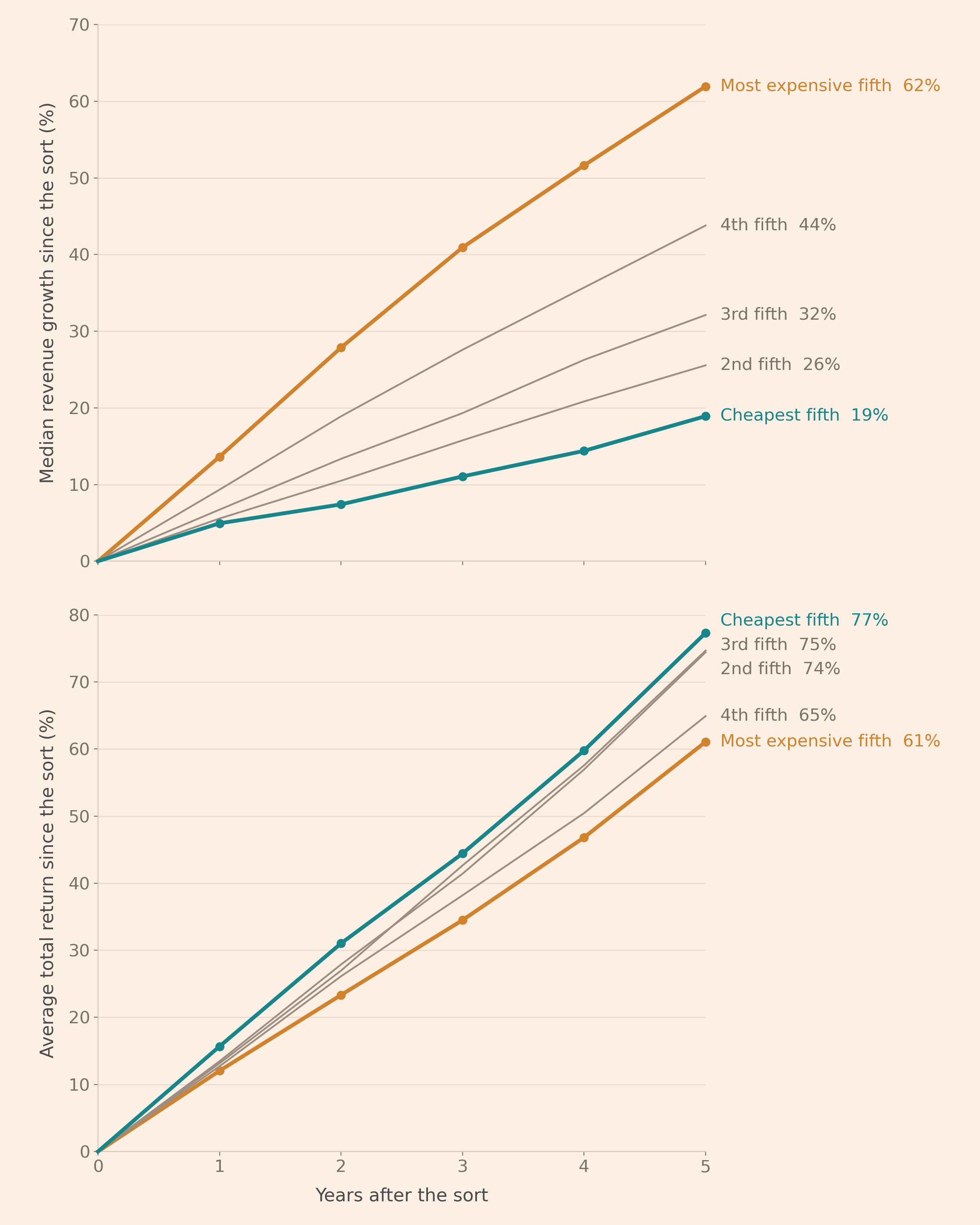
In the top panel, the orange line, the most expensive fifth, is at 62% after five years, and the teal line, the cheapest fifth, at 19%, with the three grey lines, the middle fifths, between them in order. In the bottom panel the order is reversed: the teal line is the highest, at 77%, and the orange line the lowest, at 61%. So, the fifth with the highest median growth had the lowest average return.
Limitations
Growth is measured only on the companies that stayed. The returns include the companies that left, so the growth in the top panel of the chart covers fewer of each fifth’s companies than the return in the bottom panel. What shareholders received after a delisting is not in the data. For a company taken over for cash, the last price is close to the price paid; the shareholders of a company that failed may have received less than its last price, so the return of a fifth with more failures may be overstated.
The size of the gap depends on the weighting. Weighted by market value, the most expensive fifth returned more in the sorts of 2014 to 2020, because in those years the largest companies returned more than the rest in every fifth, and more so in the most expensive fifth than in the cheapest: 99.0% weighted by market value against 64.4% with equal weights, and 88.9% against 71.7%.
The returns are raw. They are before costs and taxes, and not adjusted for risk, so the cheapest fifth may have earned more for bearing more risk, an explanation this test does not examine.
Revenue growth is not growth per share. Revenue growth includes revenue bought with acquisitions, and a company that issues shares to pay for them grows its revenue faster than its revenue per share.
The windows overlap. The five-year window after the 2010 sort shares four years with the one after the 2011 sort, so the 20 sorts are not 20 independent observations, and I do not attach confidence intervals to the differences between the fifths.
Conclusion
Did the expensive companies grow faster? Yes, about three times as fast: the median company in the most expensive fifth grew its revenue by 10.1% a year, against 3.5% in the cheapest fifth. Did their shareholders earn more? No: with an equal amount invested in each company, the most expensive fifth returned 10.0% a year and the cheapest fifth 12.1%, and the cheapest fifth returned more in 13 of the 20 sorts.
Lakonishok, Shleifer and Vishny (1994) found the same pattern in US stocks from 1968 to 1990. Their explanation, which this test does not examine, is that investors extrapolate past growth too far and pay a price that assumes more growth than the companies deliver. The takeaway is that paying for growth is not the same as getting paid for it.
Appendix: the data
The code below runs first. It reads the stock data, builds the fifths, downloads the revenue and looks up the revenue known at each sort.
Settings
The block below sets the files, the choices of the test and the chart colours. The sorts are on the last trading day of each year from 2001 to 2020, because the file has no enterprise value in 2000.
from pathlib import Path
import time

import matplotlib.pyplot as plt
import numpy as np
import pandas as pd

FOLDER = Path.cwd()                                # files are read and written beside this notebook
STOCKS_FILE = FOLDER / "Data" / "US_stocks.csv"   # one row per stock and day, from LSEG
SECTORS_FILE = FOLDER / "Data" / "US_sectors.csv"  # one sector per stock, from LSEG
COMPANIES_FILE = FOLDER / "Data" / "US_companies.csv"  # each code's company
REVENUE_FILE = FOLDER / "nr77_revenue.csv"          # downloaded once below, then read
CURRENCY_FILE = FOLDER / "nr77_revenue_currency.csv"  # the currency of that revenue, the same way
CHART_FILE = FOLDER / "growth_in_growth_stocks.png"

FIRST_YEAR, LAST_YEAR = 2001, 2020       # the sorts, one at each year-end
LARGEST = 1000                           # the largest companies by market value at each sort
EBIT_LAG = 2                             # trading days before the sort from which EBIT is taken
HORIZONS = [1, 2, 3, 4, 5]               # years after the sort, the points of the chart's lines
TABLE_HORIZONS = [1, 3, 5]               # the years in the growth table
REPORT_LAG = pd.DateOffset(months=3)     # a fiscal year's revenue counts 3 months after its end,
FRESH = pd.DateOffset(months=16)         # and only while that year ended within the last 16 months
DAYS_APART = 92                          # an h-year growth: fiscal years h years apart, +-92 days
EXTREME = 50                             # a daily return beyond +-50% must show in the market value

# The revenue download: LSEG's total revenue of each fiscal year since 1985. EDate works as a
# reporting cut-off, so 2026-09-30 includes the years that ended in late 2025 and were reported
# in 2026
REVENUE_FIELDS = ["TR.F.TotRevenue.date", "TR.F.TotRevenue"]
CURRENCY_FIELDS = ["TR.F.TotRevenue.date", "TR.F.TotRevenue.currency"]
REVENUE_PARAMETERS = {"SDate": "1985-01-01", "EDate": "2026-09-30", "Frq": "FY"}
BATCH_SIZE, SAVE_EVERY = 10, 100         # stocks per request; batches between two saves

# The five fifths, numbered 0 to 4, from the cheapest to the most expensive
GROUPS = ["Cheapest", "2nd", "3rd", "4th", "Most expensive"]

# The site's chart colours: the cream background, the text, the light grid lines, the pale frame,
# the axis labels and the tick labels, then the lines
BG, INK, GRID, SPINE = "#FCEFE3", "#1f1f1f", "#EADCCC", "#D5C6B4"
AXIS_TEXT, TICK = "#4a4a4a", "#7a7168"
TEAL, ORANGE, GREY = "#17868A", "#D2822B", "#9C8F82"
Stock data
US_stocks.csv has one row per stock and trading day, with the stock’s LSEG code in Instrument. I read the seven columns the test needs: the code, the date, the company’s market value and enterprise value, both in USD millions, its EBIT, the day’s total return in % and the day’s value traded. A trading day is a date with rows for at least 500 stocks, each sort uses the last trading day of its year, and a stock has left the data on the day its rows stop. The block also computes each stock’s median daily value traded over the year up to the sort, used below to choose between a company’s codes.
# Text columns are read as "category", which stores each different text once, and the five
# numbers as float32 rather than float64, which halves their memory: about 0.8 GB in all
stocks = pd.read_csv(STOCKS_FILE,
                     usecols=["Instrument", "Date", "Company Market Cap", "EBIT",
                              "Enterprise Value (Daily Time Series)", "Daily Total Return",
                              "Daily Value Traded"],
                     dtype={"Instrument": "category", "Date": "category",
                            "Company Market Cap": "float32", "EBIT": "float32",
                            "Enterprise Value (Daily Time Series)": "float32",
                            "Daily Total Return": "float32", "Daily Value Traded": "float32"})
# usecols keeps the file's order of columns, so rename() maps each old name to its new name
stocks = stocks.rename(columns={"Instrument": "ric", "Date": "date",
                                "Company Market Cap": "market_value", "EBIT": "ebit",
                                "Enterprise Value (Daily Time Series)": "enterprise_value",
                                "Daily Total Return": "total_return",
                                "Daily Value Traded": "value_traded"})

# The dates are text written year-month-day, so sorting them as text puts them in date order, and
# ordered categories let min() and max() find each stock's first and last day
stocks["date"] = stocks["date"].cat.reorder_categories(sorted(stocks["date"].cat.categories),
                                                       ordered=True)
# Each stock's rows must be in date order. shift() moves a column down one row, so each row sees
# the row before, and same_stock marks the rows that follow a row of the same stock. cat.codes
# numbers the dates 0, 1, 2, ... in date order, and diff() takes each row minus the row before
same_stock = stocks["ric"].eq(stocks["ric"].shift())
assert (stocks["date"].cat.codes.diff()[same_stock] > 0).all(), "a stock's days are out of order"

# The trading days: value_counts counts the rows of each date, and the dates with at least 500
# rows are kept. Then the last trading day of each year up to 2025 (the file ends in February
# 2026): groupby(...year) puts the days of each year together, and max() takes the latest
rows_per_date = stocks["date"].value_counts()
trading_days = pd.to_datetime(rows_per_date.index[rows_per_date >= 500].astype(str)).sort_values()
year_end = pd.Series(trading_days, index=trading_days).groupby(trading_days.year).max()
year_end = year_end.loc[year_end.index <= 2025]
# Each stock's first and last day; observed=True skips codes without rows, and astype(str) turns
# the categories back into text, which to_datetime reads as dates
first_day = pd.to_datetime(stocks.groupby("ric", observed=True)["date"].min().astype(str))
last_day = pd.to_datetime(stocks.groupby("ric", observed=True)["date"].max().astype(str))
first_day.index, last_day.index = first_day.index.astype(str), last_day.index.astype(str)

# The rows of the year-ends, as a small table of their own: isin marks the rows whose date is one
# of the year-ends, and str[:4] takes the first four characters of the date, the year
on_year_end = stocks["date"].isin(year_end.dt.strftime("%Y-%m-%d"))
panel = stocks.loc[on_year_end].astype({"ric": str, "date": str})
panel["year"] = panel["date"].str[:4].astype(int)
# duplicated marks a row whose stock and year came up before
assert not panel.duplicated(["ric", "year"]).any(), "a stock has two rows on one year-end"
assert panel.loc[panel["year"] == 2000, "enterprise_value"].isna().all(), "the file has EV in 2000"
# Each stock's median daily value traded over its year up to and including the year's sort day,
# known at the sort, which picks the most traded of a company's codes below. The dates are numbered
# in date order, each number's date and year come from its text, and a row after its year's sort
# day, or in a year without a sort, is left out; groupby on the numbers keeps the memory small
date_values = pd.to_datetime(pd.Series(stocks["date"].cat.categories.astype(str))).to_numpy()
date_number = stocks["date"].cat.codes.to_numpy()
row_year = pd.DatetimeIndex(date_values).year.to_numpy()[date_number]
sort_day_of_year = year_end.reindex(np.arange(row_year.min(), row_year.max() + 1)).to_numpy()
up_to_sort = date_values[date_number] <= sort_day_of_year[row_year - row_year.min()]
traded = (pd.Series(np.where(up_to_sort, stocks["value_traded"].to_numpy(), np.nan))
          .groupby([stocks["ric"].cat.codes.to_numpy(), row_year]).median())
ric_names = stocks["ric"].cat.categories.astype(str)[traded.index.get_level_values(0)]
traded.index = pd.MultiIndex.from_arrays([ric_names, traded.index.get_level_values(1)])
panel_keys = pd.MultiIndex.from_arrays([panel["ric"], panel["year"]])
panel["value_traded"] = traded.reindex(panel_keys).to_numpy()

# {:,} writes commas between thousands, and {:%d %b %Y} writes a date as 03 Jan 2000
print(f"{len(stocks):,} rows of {len(last_day):,} stocks, {len(trading_days):,} trading days "
      f"from {trading_days[0]:%d %b %Y} to {trading_days[-1]:%d %b %Y}")
sorted_panel = panel.loc[panel["year"].between(FIRST_YEAR, LAST_YEAR)]
print(f"Stocks with a market value on the year-ends {FIRST_YEAR}-{LAST_YEAR}: "
      f"{sorted_panel.groupby('year')['market_value'].count().min():,} to "
      f"{sorted_panel.groupby('year')['market_value'].count().max():,}")
print(f"Stocks whose rows stop before the file's last day: {(last_day < trading_days[-1]).sum():,}")
33,379,599 rows of 14,951 stocks, 6,574 trading days from 03 Jan 2000 to 27 Feb 2026
Stocks with a market value on the year-ends 2001-2020: 4,446 to 5,373
Stocks whose rows stop before the file's last day: 10,604EBIT at each sort
The file’s EBIT is the operating earnings of the latest twelve months, and it changes when a report is published. Each sort takes its EBIT from two trading days before the year-end, so that a report published on the sort day, or recorded a day early, is not used.
# Each year-end takes its EBIT from EBIT_LAG trading days earlier. position numbers the trading
# days 0, 1, 2, ..., and map finds, for each year-end, the trading day EBIT_LAG places before it
position = pd.Series(range(len(trading_days)), index=trading_days)
ebit_day = year_end.map(lambda day: trading_days[position.loc[day] - EBIT_LAG])
on_ebit_day = stocks["date"].isin(ebit_day.dt.strftime("%Y-%m-%d"))
earlier = stocks.loc[on_ebit_day, ["ric", "date", "ebit"]].astype({"ric": str, "date": str})
earlier["year"] = earlier["date"].str[:4].astype(int)
# merge with how="left" keeps every year-end row, and a stock without a row EBIT_LAG days earlier
# gets no EBIT; suffixes names the two EBIT columns
panel = panel.merge(earlier[["ric", "year", "ebit"]], on=["ric", "year"], how="left",
                    suffixes=("_on_the_day", ""))
both = panel[["ebit_on_the_day", "ebit"]].dropna()
print(f"EBIT taken {EBIT_LAG} trading days before each year-end differs from the year-end's own "
      f"for {(both['ebit_on_the_day'] != both['ebit']).sum():,} of {len(both):,} stock-year-ends")
EBIT taken 2 trading days before each year-end differs from the year-end's own for 600 of 114,656 stock-year-endsCumulative log returns at each year-end
For the returns of the fifths, each stock’s daily total returns add up, in logarithms, into its cumulative log return, and its cumulative log return at each year-end is kept. On days when both moves are below 20%, the daily return should move with the day’s change in the company’s market value, and the block checks that the two are correlated: the correlation is 0.96. A few returns are data errors, such as a reverse split recorded as a gain, so a daily return beyond ±50% counts only if the market value moved at least half as much in the same direction, and a return below −100% never counts; a return left out counts as 0% that day, as does a missing one. After a stock’s last day its cumulative log return stays where it was, as if the money were held in cash without interest.
# The day's change in the company's market value, in %; shift(1) within each stock takes the day
# before, so a stock's first day has none
value_before = stocks.groupby("ric", observed=True)["market_value"].shift(1)
value_change = 100 * (stocks["market_value"] / value_before - 1)
reported = stocks["total_return"]
# Ordinary days, both moves below 20%: corr is the correlation of the two columns, 1 if they agree
ordinary = reported.abs().lt(20) & value_change.abs().lt(20)
agreement = reported.loc[ordinary].corr(value_change.loc[ordinary])
assert agreement > 0.9, "the daily return does not follow the market value"
# :.2f writes a number with two decimals
print(f"Correlation of the daily return and the change in market value on ordinary days: "
      f"{agreement:.2f}")

# A move beyond EXTREME counts only if the market value confirms it: a change in the same direction
# and at least half as large. & means and, | means or, and ~ turns True into False and back
confirmed = ((np.sign(value_change) == np.sign(reported))
             & (value_change.abs() >= reported.abs() / 2))
is_error = (reported < -100) | ((reported.abs() > EXTREME) & ~confirmed)
extreme = reported.abs() > EXTREME
print(f"Daily returns: {reported.notna().sum():,}; missing: {reported.isna().sum():,}, mostly a "
      f"stock's first day; beyond ±{EXTREME}%: {extreme.sum():,}, of which {is_error.sum():,} left "
      f"out as data errors and {(extreme & ~is_error).sum():,} kept, confirmed by the market value")
# The last day of each delisted stock, whose code has a ^: shift(-1) takes the row after, so a last
# row is one followed by another stock's row
last_row = ~stocks["ric"].eq(stocks["ric"].shift(-1))
delisted_last = reported.loc[last_row & stocks["ric"].str.contains("^", regex=False)]
# :.1% writes a share as a percentage with one decimal
print(f"Last day of the {len(delisted_last):,} delisted stocks: median return "
      f"{delisted_last.median():.2f}%, beyond ±20% in {(delisted_last.abs() > 20).mean():.1%}")

# The year of each row: the date categories' years, picked by each row's category code
category_year = stocks["date"].cat.categories.str[:4].astype(int).to_numpy(dtype=np.int16)
row_year = category_year[stocks["date"].cat.codes.to_numpy()]


def year_end_wealth(daily_returns):
    """Each stock's cumulative log return at the end of each year, from daily returns in %, a
    missing one counting as 0%. log1p(x) is log(1 + x); a total loss, the logarithm of 0, is capped
    at -50 so that sums stay finite. cumsum adds up each stock's daily log returns in
    date order, last() takes its last row of each year, unstack gives one column per year, and
    ffill(axis=1) carries a stock's last value into the years after it left the data, as cash
    without interest."""
    with np.errstate(divide="ignore"):
        log_return = np.log1p(daily_returns.fillna(0).astype(float) / 100).clip(lower=-50)
    cumulative = log_return.groupby(stocks["ric"], observed=True).cumsum()
    table = (pd.DataFrame({"ric": stocks["ric"], "year": row_year, "wealth": cumulative})
             .groupby(["ric", "year"], observed=True)["wealth"].last()
             .unstack("year").reindex(columns=range(2000, 2026)).ffill(axis=1))
    table.index = table.index.astype(str)
    return table


# where() leaves the errors missing, so they count as 0%
wealth = year_end_wealth(reported.where(~is_error))
print(f"Days left out: {(is_error & (reported < 0)).sum():,} falls and "
      f"{(is_error & (reported > 0)).sum():,} rises")
del value_before, value_change, ordinary, confirmed, extreme, last_row, row_year
Correlation of the daily return and the change in market value on ordinary days: 0.96
Daily returns: 33,376,072; missing: 3,527, mostly a stock's first day; beyond ±50%: 15,394, of which 2,718 left out as data errors and 12,676 kept, confirmed by the market value
Last day of the 10,618 delisted stocks: median return 0.00%, beyond ±20% in 6.9%
Days left out: 455 falls and 2,263 risesThe 1,000 largest companies and the fifths
At each sort, in this order:
- Preference shares are left out, because they carry their company’s market value, so the company would count twice.
- Funds, the stocks without a sector that never have an EBIT, are left out.
- A company with two codes keeps one, chosen with what is known at the sort: a code with EBIT and enterprise value, then the most traded over the year, then the one with the longest history.
- Codes of different companies with the same market value on the sort day are one company’s data under two IDs when their EBIT and enterprise value match too, and one of them is kept; otherwise all of them are left out, because the market value belongs to only one company.
- The 1,000 largest by market value remain.
- The financials are left out.
- The profitable companies are cut into fifths within the year by
\[\text{EV/EBIT}_{i,t} = \frac{EV_{i,t}}{EBIT_{i,t}}.\]
The sectors are LSEG’s latest, and a code’s company is LSEG’s organization ID today, so a company whose sector or ID changed could be placed differently than it would have been at the sort.
# Each stock's sector, with its RIC as the index, so that map() can look the sectors up
sectors = pd.read_csv(SECTORS_FILE).set_index("Instrument")["Sector"]
assert sectors.index.is_unique, "a stock has two rows in the sector file"
assert last_day.index.isin(sectors.index).all(), "a stock is missing from the sector file"
# Whether a stock ever has an EBIT: count() counts the values that are present
has_ebit = stocks.groupby("ric", observed=True)["ebit"].count() > 0
has_ebit.index = has_ebit.index.astype(str)
del stocks, same_stock          # free the memory of the daily data

# Each code's company, LSEG's organization ID, from the company file; a code without one counts
# as a company of its own
company_of = pd.read_csv(COMPANIES_FILE, dtype=str).set_index("Instrument")["Company"]
# The order in which a company's codes are preferred, all known at the sort: a code with EBIT and
# EV, then the most traded over the year, then the one with the longest history, then by name
ORDER, ASCENDING = ["complete", "value_traded", "first", "ric"], [False, False, True, True]
counts, tables, kept_from_shared = [], [], 0
for year in range(FIRST_YEAR, LAST_YEAR + 1):
    day = panel.loc[(panel["year"] == year) & panel["market_value"].notna()]
    count = {"year": year, "with a market value": len(day)}
    # str.contains marks the codes with _p in them; map looks each code up in sectors and has_ebit,
    # isna() marks the codes without a sector, and ~ turns True into False and back
    preference = day["ric"].str.contains("_p", regex=False)
    fund = day["ric"].map(sectors).isna() & ~day["ric"].map(has_ebit)
    count["preference shares"], count["funds"] = preference.sum(), (fund & ~preference).sum()
    day = day.loc[~preference & ~fund]

    # One code per company, by LSEG's organization ID; a code without one is a company of its own.
    # sort_values puts the preferred code first within each company, and drop_duplicates keeps it
    day = day.assign(company=day["ric"].map(company_of).fillna(day["ric"]),
                     complete=day["ebit"].notna() & day["enterprise_value"].notna(),
                     first=day["ric"].map(first_day))
    chosen = (day.sort_values(["company"] + ORDER, ascending=[True] + ASCENDING)
              .drop_duplicates("company"))
    count["second codes"] = len(day) - len(chosen)
    day = chosen
    # Codes of different companies with the same market value that day: one company's data under
    # two IDs if their EBIT and EV match too, kept once in the same order; otherwise the value
    # belongs to only one of them, and both are left out. duplicated(keep=False) marks every row
    # whose value appears more than once, and nunique(dropna=False) == 1 means the values match
    shared = day.loc[day["market_value"].duplicated(keep=False)]
    keep = []
    for value, same in shared.groupby("market_value"):
        same_ebit = same["ebit"].nunique(dropna=False) == 1
        same_ev = same["enterprise_value"].nunique(dropna=False) == 1
        if same_ebit and same_ev:
            keep.append(same.sort_values(ORDER, ascending=ASCENDING).index[0])
    kept_from_shared += len(keep)
    left_out = shared.index.difference(keep)          # the rows of shared that are not kept
    count["shared market value"] = len(left_out)
    day = day.drop(left_out)
    assert not day["company"].duplicated().any(), f"a company has two codes in {year}"
    assert not day["market_value"].duplicated().any(), f"two codes share a market value in {year}"

    # nlargest keeps the rows with the largest market values; copy() makes a table of its own
    largest = day.nlargest(LARGEST, "market_value").copy()
    assert len(largest) == LARGEST, f"fewer than {LARGEST} companies in {year}"
    financial = largest["ric"].map(sectors) == "Financials"
    count["financials"] = financial.sum()
    largest = largest.loc[~financial]
    has_values = largest["ebit"].notna() & largest["enterprise_value"].notna()
    profitable = has_values & (largest["ebit"] > 0)
    assert (largest.loc[profitable, "enterprise_value"] > 0).all(), "EV of zero or less, EBIT above"
    count["no EV or EBIT"] = (~has_values).sum()
    count["loss-making"] = (has_values & (largest["ebit"] <= 0)).sum()
    count["in the fifths"] = profitable.sum()

    # EV/EBIT in float64, so that the ranking uses the full precision of the ratio
    largest["ev_ebit"] = largest["enterprise_value"].astype(float) / largest["ebit"].astype(float)
    # rank(method="first") numbers the profitable companies 1, 2, 3, ... from the lowest EV/EBIT,
    # ties in the order they come, and qcut cuts the numbers into five equal parts, 0 to 4
    largest["group"] = np.nan
    ev_ebit_rank = largest.loc[profitable, "ev_ebit"].rank(method="first")
    largest.loc[profitable, "group"] = pd.qcut(ev_ebit_rank, 5, labels=False)
    counts.append(count)
    tables.append(largest)

# The companies sorted, one row per company and sort, with its group: concat stacks the 20 tables,
# and ignore_index numbers the rows anew
universe = pd.concat(tables, ignore_index=True)
counts = pd.DataFrame(counts).set_index("year")
# What the sorts left out, added up over the 20 sorts: sum() adds up each column
totals = counts.sum()
print(f"Over the {len(counts)} sorts, {totals['with a market value']:,} codes had a market value. "
      f"Left out before taking the {LARGEST:,} largest: {totals['preference shares']:,} preference "
      f"shares, {totals['funds']:,} funds, {totals['second codes']:,} second codes of a company "
      f"and {totals['shared market value']:,} codes sharing a market value with another company's")
# :.0f rounds a number to a whole number
print(f"Of the {LARGEST * len(counts):,} company-sorts among the {LARGEST:,} largest: "
      f"{totals['financials']:,} financials, {totals['no EV or EBIT']:,} without EV or EBIT and "
      f"{totals['loss-making']:,} loss-making are left out, and {totals['in the fifths']:,} are in "
      f"the fifths, {counts['in the fifths'].min() / 5:.0f} to "
      f"{counts['in the fifths'].max() / 5:.0f} companies per fifth")
# The company-sorts whose EBIT on the sort day itself differs from the one used, taken two trading
# days earlier
lagged = universe[["ebit_on_the_day", "ebit"]].dropna()
print(f"Company-sorts whose EBIT on the sort day differs from the one used: "
      f"{(lagged['ebit_on_the_day'] != lagged['ebit']).sum()} of {len(lagged):,}")
Over the 20 sorts, 96,857 codes had a market value. Left out before taking the 1,000 largest: 550 preference shares, 733 funds, 576 second codes of a company and 98 codes sharing a market value with another company's
Of the 20,000 company-sorts among the 1,000 largest: 2,938 financials, 710 without EV or EBIT and 1,046 loss-making are left out, and 15,306 are in the fifths, 134 to 163 companies per fifth
Company-sorts whose EBIT on the sort day differs from the one used: 24 of 16,883Revenue from LSEG
The block downloads each stock’s total revenue for each fiscal year since 1985, dated at the end of the fiscal year, and, for the companies sorted, the currency of that revenue. Each download runs once and saves to a file beside the notebook; a later run reads the file and downloads only the stocks it lacks. The stocks go in batches of 10 with a pause of one second, each request gets three attempts with a longer wait after each failure, a batch that still fails is tried one stock at a time, the file is saved every 100 batches, and if a stock fails all its attempts, the run ends with an error after saving the rest.
def open_lseg():
    """Open the LSEG session. lseg-data 2.1.1 passes proxy={} to httpx, which httpx 0.28 and later
    reject with "'dict' object has no attribute 'url'"; on that error the empty dictionary is turned
    into no proxy, and the session is opened again."""
    import httpx
    import lseg.data as ld
    ld.get_config().set_param("http.request-timeout", 300)    # seconds; read when the session opens
    try:
        ld.open_session()
    except AttributeError:
        for client in (httpx.Client, httpx.AsyncClient):
            if not getattr(client.__init__, "_lseg_patched", False):
                def patched(original):
                    def __init__(self, *args, **kwargs):
                        if isinstance(kwargs.get("proxy"), dict):
                            kwargs["proxy"] = next((value for value in kwargs["proxy"].values()
                                                    if value), None)
                        return original(self, *args, **kwargs)
                    __init__._lseg_patched = True
                    return __init__
                client.__init__ = patched(client.__init__)
        ld.open_session()


def download(ld, batch, fields):
    """The fields for a list of RICs, or None if all three attempts fail."""
    for attempt in range(3):
        try:
            return ld.get_data(batch, fields, REVENUE_PARAMETERS)
        except Exception as error:
            print(f"  a batch of {len(batch)} stocks: attempt {attempt + 1} failed: "
                  f"{type(error).__name__}")
            time.sleep(2 * 2 ** attempt)             # wait 2, then 4, then 8 seconds
    return None


def save(tables, path, columns):
    """Append the downloaded tables to the file and return the number of rows added. A stock
    without data keeps its one empty row, so a later run knows it was asked for."""
    chunk = pd.concat(tables, ignore_index=True)
    assert chunk.shape[1] == len(columns), f"expected {columns}, got {list(chunk.columns)}"
    chunk.columns = columns
    chunk = chunk.drop_duplicates()
    # mode="a" appends to the file; the column names are written only when the file is new
    chunk.to_csv(path, mode="a", index=False, header=not path.exists())
    return len(chunk)


def download_all(rics, fields, path, columns):
    """Download the fields of every RIC that the file at path lacks, in batches of BATCH_SIZE,
    trying a failed batch one stock at a time and saving every SAVE_EVERY batches. A stock that
    fails all its attempts stops the run."""
    saved = set()
    if path.exists():
        saved = set(pd.read_csv(path, usecols=["Instrument"])["Instrument"])
    missing = [ric for ric in rics if ric not in saved]
    print(f"{path.name}: {len(saved):,} stocks already saved, {len(missing):,} to download")
    if not missing:
        return
    import lseg.data as ld                       # needs LSEG Workspace running and logged in
    open_lseg()                                  # defined above, with the httpx fix
    # The batches: missing[0:10], missing[10:20], and so on; a slice stops before its end
    batches = [missing[first:first + BATCH_SIZE] for first in range(0, len(missing), BATCH_SIZE)]
    waiting, failed, saved_rows = [], [], 0
    for number, batch in enumerate(batches, start=1):    # enumerate counts the batches from 1
        table = download(ld, batch, fields)
        if table is not None:
            waiting.append(table)
        else:
            for ric in batch:                    # one stock at a time
                single = download(ld, [ric], fields)
                if single is None:
                    failed.append(ric)
                else:
                    waiting.append(single)
        time.sleep(1)
        if (number % SAVE_EVERY == 0 or number == len(batches)) and waiting:
            saved_rows += save(waiting, path, columns)
            waiting = []
            print(f"batch {number:,} of {len(batches):,}: {saved_rows:,} rows saved")
    ld.close_session()
    print(f"Done: {saved_rows:,} rows added")
    # The rows saved so far stay in the file, and a later run asks only for the stocks it lacks
    assert not failed, f"{len(failed)} stocks failed to download: run the cell again"


download_all(last_day.index.tolist(), REVENUE_FIELDS, REVENUE_FILE,
             ["Instrument", "Date", "Revenue"])
download_all(universe["ric"].unique().tolist(), CURRENCY_FIELDS, CURRENCY_FILE,
             ["Instrument", "Date", "Currency"])
nr77_revenue.csv: 15,550 stocks already saved, 0 to download
nr77_revenue_currency.csv: 2,245 stocks already saved, 0 to downloadThe revenue file also holds the stocks of an earlier version of the stock file, so it has more stocks than the stock file.
Revenue known at each sort
The revenue counted as known at the sort of year \(t\) is the revenue of the latest fiscal year that ended at least three months before 31 December of year \(t\): an assumption about filing dates, since US companies normally file their annual reports within 60 to 90 days of the year end. A fiscal year that ended 16 months or more before counts as unknown. A fiscal year listed with two different figures, or in a currency other than US dollars, is left out. Looking the revenue up on 31 December, at most two days after the sort, makes every window exactly \(h\) years long. The block also checks the units: market value is in USD millions and revenue in dollars, so the median price-to-sales, the market value divided by the revenue, has to be between 0.3 and 10, a usual level.
revenue_rows = pd.read_csv(REVENUE_FILE, parse_dates=["Date"])
# The revenue file also holds stocks of earlier versions of the stock file; this file's are used
revenue_rows = revenue_rows.loc[revenue_rows["Instrument"].isin(set(last_day.index))]
asked = revenue_rows["Instrument"].nunique()
print(f"{len(revenue_rows):,} rows for {asked:,} of the {len(last_day):,} stocks")
assert asked == len(last_day), "stocks are missing from the revenue file: run the download again"
# A stock without any revenue has one row with no date and no revenue, and some fiscal years are
# listed without a revenue; dropna removes both
revenue = revenue_rows.dropna(subset=["Date", "Revenue"]).copy()
revenue.columns = ["ric", "period_end", "revenue"]
print(f"{len(revenue):,} fiscal years with revenue, for {revenue['ric'].nunique():,} stocks; "
      f"{revenue_rows['Date'].notna().sum() - len(revenue):,} fiscal years listed without one")

# A fiscal year listed twice: exact repeats are dropped once, and a year with two different
# figures is left out, since it is not clear which is right
repeats = revenue.duplicated()
revenue = revenue.loc[~repeats]
ambiguous = revenue.duplicated(["ric", "period_end"], keep=False)
assert ambiguous.sum() <= 10, "many fiscal years have two revenues: check the download"
revenue = revenue.loc[~ambiguous].sort_values(["ric", "period_end"], ignore_index=True)
print(f"Fiscal years listed twice: {repeats.sum():,} with the same figure; "
      f"{ambiguous.sum() // 2:,} with two different figures, left out")

# The currency of each fiscal year's revenue, for the companies sorted. A year in a currency other
# than US dollars is left out, since its growth and price-to-sales could mix currencies
currency = pd.read_csv(CURRENCY_FILE, parse_dates=["Date"]).dropna(subset=["Date"])
currency.columns = ["ric", "period_end", "currency"]
currency = currency.drop_duplicates()
assert not currency.duplicated(["ric", "period_end"]).any(), "a fiscal year has two currencies"
revenue = revenue.merge(currency, on=["ric", "period_end"], how="left")
of_sorted = revenue["ric"].isin(universe["ric"])
in_dollars = of_sorted & (revenue["currency"] == "USD")
# A year of a sorted company in another currency, or without one, is left out
not_dollars = of_sorted & ~in_dollars
print(f"Fiscal years of the sorted companies: {of_sorted.sum():,}; in US dollars "
      f"{in_dollars.sum():,}; left out: {(not_dollars & revenue['currency'].notna()).sum():,} in "
      f"another currency and {(not_dollars & revenue['currency'].isna()).sum():,} without one")
revenue = revenue.loc[~not_dollars].drop(columns="currency").reset_index(drop=True)

# Revenue is looked up on 31 December of each year to 2025, so that every window is exactly h years
# long; the three years before the first sort are looked up but not used in this post. The sort
# itself is on the year's last trading day, at most two days earlier
dates = pd.DataFrame({"year": range(FIRST_YEAR - 3, 2026)})
dates["date"] = pd.to_datetime(dates["year"].astype(str) + "-12-31")
# One row for each stock ever sorted and each of those dates: unique() lists each code once, and
# merge with how="cross" pairs every code with every date
queries = pd.DataFrame({"ric": universe["ric"].unique()}).merge(dates, how="cross")


def latest_revenue(queries, lag, fresh):
    """For each stock and date in queries, the revenue of the latest fiscal year that counted by
    that date, `lag` after the year ended, and the end of that year; missing when that year ended
    `fresh` or longer before the date. merge_asof finds, for each date, the last fiscal year that
    counted at or before it, within the same stock (by="ric")."""
    years = revenue[["ric", "period_end", "revenue"]]
    years = years.assign(counts_from=years["period_end"] + lag)
    found = pd.merge_asof(queries.sort_values("date"), years.sort_values("counts_from"),
                          left_on="date", right_on="counts_from", by="ric", direction="backward")
    stale = found["period_end"] <= found["date"] - fresh
    found.loc[stale, ["period_end", "revenue"]] = np.nan
    return found.set_index(["ric", "year"])[["period_end", "revenue"]]


def revenue_growth(table, known, horizon):
    """The log growth of known revenue from each row's sort to `horizon` years later, and the
    reason when it cannot be measured. np.select takes, row by row, the first condition that
    holds."""
    # reindex looks up each row's stock and year in known; a pair that known lacks gets missing
    # values, and to_numpy() gives the plain values without the index
    start = known.reindex(pd.MultiIndex.from_arrays([table["ric"], table["year"]]))
    end = known.reindex(pd.MultiIndex.from_arrays([table["ric"], table["year"] + horizon]))
    start_revenue, end_revenue = start["revenue"].to_numpy(), end["revenue"].to_numpy()
    # A stock has left the data when its rows stop before the last trading day of year t + h
    last = table["ric"].map(last_day).to_numpy()
    left = last < (table["year"] + horizon).map(year_end).to_numpy()
    # The days between the two fiscal year ends, dividing by one day, against h years of 365.25 days
    apart = (end["period_end"].to_numpy() - start["period_end"].to_numpy()) / np.timedelta64(1, "D")
    # ~(x > 0) is True for a missing revenue too, because a comparison with a missing value is False
    status = np.select([left, ~(start_revenue > 0), ~(end_revenue > 0),
                        ~(np.abs(apart - 365.25 * horizon) <= DAYS_APART)],
                       ["left the data", "no revenue at the start", "no revenue at the end",
                        "fiscal years not h years apart"], default="measured")
    with np.errstate(divide="ignore", invalid="ignore"):     # logarithms of missing values
        growth = np.where(status == "measured", np.log(end_revenue / start_revenue), np.nan)
    return pd.DataFrame({"status": status, "growth": growth}, index=table.index)


known = latest_revenue(queries, REPORT_LAG, FRESH)
at_sort = known.reindex(pd.MultiIndex.from_arrays([universe["ric"], universe["year"]]))
universe["sales"] = at_sort["revenue"].to_numpy()
universe["price_to_sales"] = universe["market_value"].astype(float) * 1e6 / universe["sales"]
with_sales = universe["sales"] > 0
median_price_to_sales = universe.loc[with_sales, "price_to_sales"].median()
assert 0.3 < median_price_to_sales < 10, "price-to-sales is far from usual levels: check the units"
print(f"Median price-to-sales at the sorts: {median_price_to_sales:.2f}")
# The mean of True and False values is the share that is True
coverage = 100 * with_sales.groupby(universe["year"]).mean()
print(f"Companies sorted with revenue known at the sort: {coverage.min():.0f}% to "
      f"{coverage.max():.0f}% of a sort's companies")
238,997 rows for 14,951 of the 14,951 stocks
228,302 fiscal years with revenue, for 13,101 stocks; 8,845 fiscal years listed without one
Fiscal years listed twice: 0 with the same figure; 1 with two different figures, left out
Fiscal years of the sorted companies: 52,950; in US dollars 52,815; left out: 135 in another currency and 0 without one
Median price-to-sales at the sorts: 2.17
Companies sorted with revenue known at the sort: 96% to 99% of a sort's companiesRead next
- The Magic Formula worked. Just not lately. Another sort of US stocks on EBIT relative to price, and what it returned.
- The most profitable US companies beat the S&P 500, and the least profitable lost money. A sort of US stocks by profitability instead of price.
- Do large stocks crash more often after doubling? What followed large gains in single US stocks.
Disclaimer: an empirical study for discussion purposes, not investment advice. The design is descriptive and not causal. Past performance does not guarantee future returns.
Sources: Josef Lakonishok, Andrei Shleifer and Robert W. Vishny, “Contrarian Investment, Extrapolation, and Risk”, Journal of Finance 49(5), 1541 to 1578 (1994). Daily market values, enterprise values, EBIT and total returns of US-incorporated stocks, and each company’s revenue by fiscal year, from LSEG Workspace (licensed); I do not reproduce the raw data here.