How to read logit and probit coefficients as changes in the probability of a crime.
Published
September 20, 2026
Say we have 20,000 company announcements and, in truth, a market crime happened at 2,253 of them: insider trading, meaning that somebody traded on the information before the announcement was public. We want the probability of a crime at each announcement, estimated from three variables. A straight line fitted to an outcome of 1 for a crime and 0 otherwise predicts a value below zero for about one announcement in ten.
The issue is that a probability cannot be negative. Logistic and probit regression are two models that keep the probability between 0 and 1. Their coefficients, the weights they give the variables, no longer give a fixed change in the probability. I fit the three models and explain what the logistic and probit coefficients mean for the probability of a crime. In the logistic model, one more standard deviation of the price move raises the probability of a crime from 50% to 74.6%, but from 2% only to 5.7%, so the same coefficient gives different changes in the probability.
Simulating the data
With real announcements I would not know which ones were crimes, because the records count a crime that nobody detects as no crime. Thus I simulate the announcements. Each one gets three variables, drawn from the standard normal distribution, which is bell-shaped with an average of 0 and a standard deviation of 1. So one unit of a variable is one standard deviation, a measure of how far values typically are from their average:
information_value, the size of the price move the announcement caused, with a positive coefficient, because a larger move means a larger profit from trading ahead of the announcement.
insiders_with_access, how far the number of people who knew beforehand is above or below the average, with a positive coefficient.
largest_order, the size of the largest order placed before the announcement, correlated with information_value and with a negative coefficient, on the assumption that an offender avoiding attention splits a large order into small ones.
A crime happens at random, with a probability that increases with the first two variables and decreases with the third, through coefficients I set. The models never receive these coefficients, so I can compare the logistic estimates with the coefficients I set. I fit every model to these 20,000 announcements, the fitting sample. The box below gives the formula and the code.
NoteHow the announcements are simulated
The true score of announcement \(i\) combines the three variables with the coefficients I set,
where \(x_1\), \(x_2\) and \(x_3\) are information_value, insiders_with_access and largest_order, and \(x_1\), \(x_2\) and \(u_i\) are independent standard normal draws, so \(x_3\) has a standard deviation of 1, since \(0.8^2 + 0.6^2 = 1\), and a correlation of 0.8 with \(x_1\), on a scale from −1 to 1 on which 1 would mean that the two move in perfect step. The block below turns each score into a probability of a crime with the logistic function, \(p_i = e^{\eta_i}/(1 + e^{\eta_i})\), which a later section explains: an announcement with all three variables at 0 has a score of \(-2.4\) and a probability of \(e^{-2.4}/(1 + e^{-2.4}) = 8.3\%\). The block then decides at random whether a crime happens, with that probability, independently across announcements. The simulation draws 30,000 announcements. This post fits the models to the first 20,000, and a second post tests the logistic model’s probabilities on the last 10,000.
import numpy as npimport pandas as pdN_ANNOUNCEMENTS =30000N_FITTING =20000# the other 10,000 are the test samplerng = np.random.default_rng(11) # fixed, so every number in the post reproducesinformation_value = rng.normal(0, 1, N_ANNOUNCEMENTS)insiders_with_access = rng.normal(0, 1, N_ANNOUNCEMENTS)# 0.8 squared plus 0.6 squared is 1, so largest_order is drawn with a standard deviation of 1,# like the other two variables, and a correlation of 0.8 with information_value.largest_order =0.8* information_value +0.6* rng.normal(0, 1, N_ANNOUNCEMENTS)variables = pd.DataFrame({"information_value": information_value,"insiders_with_access": insiders_with_access,"largest_order": largest_order})# The coefficients I set, which I never give to a model below. Each one is a coefficient on# the log odds, which the logistic-model section derives.TRUE_INTERCEPT =-2.4TRUE_VARIABLE_COEFFICIENTS = {"information_value": 1.1, "insiders_with_access": 0.7,"largest_order": -0.5}VARIABLE_NAMES =list(TRUE_VARIABLE_COEFFICIENTS.keys())def logistic_function(score):"""Convert any score into a probability between 0 and 1. A score of 0 gives 0.50, a score of -4 gives about 0.02, and a score of 4 about 0.98. """return1.0/ (1.0+ np.exp(-score))# For each announcement, multiply each variable by its coefficient and add the three# products, then pass that sum through the logistic function to get a probability.true_coefficients = np.array(list(TRUE_VARIABLE_COEFFICIENTS.values()))true_score = TRUE_INTERCEPT + variables.to_numpy() @ true_coefficientstrue_probability = logistic_function(true_score)# Draw each outcome: a crime whenever a random number between 0 and 1 is below the# announcement's probability, which happens with exactly that probability.crime_draw = rng.uniform(0, 1, N_ANNOUNCEMENTS)is_crime = pd.Series((crime_draw < true_probability).astype(int))# The first 20,000 announcements are the fitting sample and the last 10,000 the test sample.# Every announcement is drawn the same way and independently of the others, so splitting by# position is equivalent to a random split.fitting_sample = np.arange(N_ANNOUNCEMENTS) < N_FITTINGtest_sample =~fitting_sample# DataFrame.loc[rows, columns] selects rows and columns; omitting columns keeps all columns.# Series.loc[rows] selects rows. Here, fitting_sample keeps the rows marked True.print(f"announcements {N_ANNOUNCEMENTS:,}, crimes {is_crime.sum():,} ({is_crime.mean():.2%})")print(f" fitting sample {fitting_sample.sum():,}, crimes {is_crime.loc[fitting_sample].sum():,} "f"({is_crime.loc[fitting_sample].mean():.2%})")print(f" test sample {test_sample.sum():,}, crimes {is_crime.loc[test_sample].sum():,} "f"({is_crime.loc[test_sample].mean():.2%})")print(f"true probability ranges from {true_probability.min():.4f} to {true_probability.max():.4f}")print(f"correlation between information_value and largest_order: "f"{np.corrcoef(information_value, largest_order)[0, 1]:.3f}")
announcements 30,000, crimes 3,425 (11.42%)
  fitting sample 20,000, crimes 2,253 (11.27%)
  test sample    10,000, crimes 1,172 (11.72%)
true probability ranges from 0.0017 to 0.8316
correlation between information_value and largest_order: 0.797
Of the 30,000 announcements, 3,425 are crimes, 11.4%: 2,253 in the fitting sample and 1,172 in the test sample. The true probabilities range from 0.0017 to 0.8316, and the correlation between information_value and largest_order is 0.797, close to the 0.8 that the formula sets.
Why not a straight line
The block below fits a straight line to the 0/1 outcome, the linear probability model, to check whether its predicted values are between 0 and 1.
import statsmodels.api as smdef with_intercept(frame):"""Put a column of ones in front of the variables. Multiplying that column by the intercept gives the intercept itself, so one matrix multiplication covers the intercept and the other coefficients together. """# start with the column of ones, then copy each variable in beside it columns = pd.DataFrame({"const": 1.0}, index=frame.index)for name in VARIABLE_NAMES: columns[name] = frame[name]return columnsdesign = with_intercept(variables)fitting_design = design.loc[fitting_sample]fitting_outcome = is_crime.loc[fitting_sample]linear = sm.OLS(fitting_outcome, fitting_design).fit()linear_prediction = linear.predict(fitting_design)print(linear.params.round(4).to_string())print(f"\npredicted values range from {linear_prediction.min():.3f} to "f"{linear_prediction.max():.3f}")print(f"below 0: {(linear_prediction <0).sum():,} of {len(linear_prediction):,} "f"({(linear_prediction <0).mean():.1%})")print(f"above 1: {(linear_prediction >1).sum():,}")
const                   0.1127
information_value       0.0971
insiders_with_access    0.0624
largest_order          -0.0457

predicted values range from -0.210 to 0.460
below 0: 2,168 of 20,000 (10.8%)
above 1: 0
Each printed coefficient is a fixed change in the predicted value: one more standard deviation of information_value adds 0.097 at every announcement. The predicted values range from −0.210 to 0.460, and 2,168 of them, 10.8% of the fitting sample, are below zero, so those 2,168 values cannot be probabilities. James and co-authors (2023) find predicted values below zero when they fit a straight line to credit card default data.
The logistic model
The logistic model keeps a weighted sum of the variables, which I call the score of an announcement:
Here \(\beta_0\) is the intercept, the score when all three variables are 0, and \(\beta_1\) to \(\beta_3\) are the coefficients on information_value, insiders_with_access and largest_order. The logistic function converts the score into a probability:
\[p = \frac{e^{\eta}}{1 + e^{\eta}}.\]
A score of 0 gives a probability of 0.50. Lower scores give probabilities closer to 0 and higher scores probabilities closer to 1, so the probability is an S-shaped function of the score, always strictly between 0 and 1.
The odds are the probability of a crime divided by the probability of no crime. A probability of 0.2 gives odds of \(0.2/0.8 = 1/4\), one crime for every four announcements without a crime. For the logistic function, dividing \(p\) by \(1 - p\) gives the odds in terms of the score:
\[\frac{p}{1 - p} = e^{\eta}.\]
Taking the natural logarithm of both sides, which undoes the exponential \(e^{\eta}\), shows that the score is the logarithm of the odds, the log odds or logit, which gives the model its name:
So a score of −2.2 gives a one-in-ten chance of a crime and −4.6 a one-in-a-hundred chance, and scores of 2.2 and 4.6 give 0.90 and 0.99.
Estimating the coefficients
I estimate the coefficients by maximum likelihood: I choose the coefficients that make the observed outcomes as likely as possible. An announcement \(i\) with outcome \(y_i\), 1 for a crime and 0 otherwise, contributes its predicted probability \(p_i\) if a crime happened and \(1 - p_i\) if not. The likelihood is the product of these contributions over the 20,000 announcements of the fitting sample. That product is too small for a computer to represent, so the fit maximises its logarithm, a sum:
The block below fits the logistic model with the statsmodels library and compares its coefficients with the coefficients I set.
# statsmodels finds the coefficients that maximise the log likelihood; disp=0 turns off the# messages it prints while it searcheslogit = sm.Logit(fitting_outcome, fitting_design).fit(disp=0)truth = np.array([TRUE_INTERCEPT] +list(TRUE_VARIABLE_COEFFICIENTS.values()))comparison = pd.DataFrame({"coefficient I set": truth,"estimate": logit.params.to_numpy()}, index=["intercept"] + VARIABLE_NAMES)print(comparison.round(4).to_string())
                      coefficient I set  estimate
intercept                          -2.4   -2.4260
information_value                   1.1    1.0774
insiders_with_access                0.7    0.6955
largest_order                      -0.5   -0.5025
The estimates are within 0.03 of the coefficients I set. The box below maximises the same sum with my own code, to show what the fit does.
NoteThe log likelihood maximised by hand
The block below codes the log likelihood, maximises it with the optimiser in SciPy and compares the result with the statsmodels coefficients.
from scipy.optimize import minimizedef negative_log_likelihood(coefficients):"""Return the negative average log likelihood of the fitting sample. The optimiser searches for the smallest value, and the smallest negative log likelihood is the largest log likelihood, so minimising this returns the maximum likelihood fit. """ score = fitting_design.to_numpy() @ coefficients probability = logistic_function(score)# np.log(0) is minus infinity, so hold the probability between 1e-12 and 1 - 1e-12 probability = np.clip(probability, 1e-12, 1-1e-12) crime_terms = fitting_outcome * np.log(probability) no_crime_terms = (1- fitting_outcome) * np.log(1- probability)# I return the mean of the terms. Dividing by the fixed number of announcements gives the# log likelihood per announcement and leaves the best coefficients unchanged.return-np.mean(crime_terms + no_crime_terms)# method="BFGS" picks one of the optimiser's search routines. Every coefficient starts at# zero, which gives every announcement a probability of 0.5.starting_values = np.zeros(fitting_design.shape[1])# stop searching once the size of the function's slope is below 1e-9by_hand = minimize(negative_log_likelihood, starting_values, method="BFGS", options={"gtol": 1e-9})# an optimiser can stop before it finds the minimum and still return coefficients, so checkassert by_hand.success, f"the optimiser did not find the minimum: {by_hand.message}"by_hand_comparison = pd.DataFrame({"my estimate": by_hand.x,"statsmodels estimate": logit.params.to_numpy()}, index=["intercept"] + VARIABLE_NAMES)print(by_hand_comparison.round(4).to_string())print(f"\noptimiser succeeded: {by_hand.success}")print(f"largest difference between my estimates and statsmodels: "f"{np.abs(by_hand.x - logit.params.to_numpy()).max():.2e}")
                      my estimate  statsmodels estimate
intercept                 -2.4260               -2.4260
information_value          1.0774                1.0774
insiders_with_access       0.6955                0.6955
largest_order             -0.5025               -0.5025

optimiser succeeded: True
largest difference between my estimates and statsmodels: 1.63e-08
My coefficients and the statsmodels coefficients differ by less than 0.000001, so my code reproduces the library’s fit.
The probit model
The probit model replaces the logistic function with the standard normal distribution function \(\Phi\), which gives the probability that a standard normal variable is below a given value:
\[p = \Phi(\eta).\]
So the same probability needs a different score in each model. A one-in-ten chance of a crime needs a score of −2.2 in the logistic model, as the odds table above shows, and −1.28 in the probit model, because a standard normal variable is below −1.28 with a probability of 10%. The block below fits the probit model to compare its coefficients and predicted probabilities with the logistic ones.
probit = sm.Probit(fitting_outcome, fitting_design).fit(disp=0)link_comparison = pd.DataFrame({"logit": logit.params.to_numpy(),"probit": probit.params.to_numpy()}, index=["intercept"] + VARIABLE_NAMES)link_comparison["logit / probit"] = link_comparison["logit"] / link_comparison["probit"]print(link_comparison.round(4).to_string())logit_probability = logit.predict(fitting_design)probit_probability = probit.predict(fitting_design)gap = (logit_probability - probit_probability).abs()# idxmax() gives the row label of the largest gap, and .loc looks up that row's probabilityprint(f"predicted probabilities differ by {gap.mean():.5f} on average and {gap.max():.4f} at most, "f"the largest at a predicted probability of {logit_probability.loc[gap.idxmax()]:.3f}")
                       logit  probit  logit / probit
intercept            -2.4260 -1.3739          1.7658
information_value     1.0774  0.5688          1.8943
insiders_with_access  0.6955  0.3661          1.8997
largest_order        -0.5025 -0.2679          1.8756
predicted probabilities differ by 0.00460 on average and 0.0661 at most, the largest at a predicted probability of 0.752
The logistic coefficients on the three variables are 1.876 to 1.900 times the probit coefficients, and the logistic intercept is 1.766 times the probit intercept. The predicted probabilities of the logistic and probit models differ by 0.0046 on average and by 0.066 at most, at an announcement with a predicted probability of 0.75. So the two models give almost the same probabilities, and a table of coefficients has to name its model.
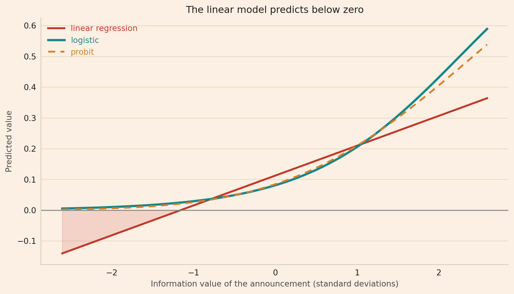
The chart below plots each model’s predicted value as information_value changes, holding the other two variables at their averages, to show the three models side by side.
Show the chart code
import matplotlib.pyplot as pltRED, TEAL, ORANGE, GREY ="#C0392B", "#17868A", "#D2822B", "#888888"# The site's chart colours: a cream background, a light grid and a pale frame, so every chart# on the site has the same look.BG, INK, GRID, SPINE, AXIS_TEXT ="#FCEFE3", "#1f1f1f", "#EADCCC", "#D5C6B4", "#4a4a4a"def style_chart(figure, axis):"""Give a finished chart the site's cream background, light grid and pale frame.""" figure.patch.set_facecolor(BG) axis.set_facecolor(BG) axis.grid(True, axis="y", color=GRID, lw=1.0) axis.set_axisbelow(True)for side in ("top", "right"): axis.spines[side].set_visible(False)for side in ("left", "bottom"): axis.spines[side].set_color(SPINE) axis.tick_params(axis="both", length=0, colors=INK, pad=6) axis.xaxis.label.set_color(AXIS_TEXT) axis.yaxis.label.set_color(AXIS_TEXT) axis.title.set_color(INK)# each legend entry in the colour of its line legend = axis.get_legend()for text, line inzip(legend.get_texts(), legend.get_lines()): text.set_color(line.get_color())# Vary information_value across the chart while holding insiders_with_access and# largest_order at their fitting-sample averages. Each curve uses the coefficients# estimated for that model, so the three differ both in the curve applied to the score and# in the coefficients inside it.low, high = np.percentile(information_value[fitting_sample], [0.5, 99.5])grid = np.linspace(low, high, 300)curve_input = pd.DataFrame({"const": 1.0,"information_value": grid,"insiders_with_access": variables.loc[fitting_sample, "insiders_with_access"].mean(),"largest_order": variables.loc[fitting_sample, "largest_order"].mean(),})figure, axis = plt.subplots(figsize=(9, 5.2))linear_curve = linear.predict(curve_input)axis.plot(grid, linear_curve, color=RED, lw=2.4, label="linear regression")axis.plot(grid, logit.predict(curve_input), color=TEAL, lw=2.8, label="logistic")axis.plot(grid, probit.predict(curve_input), color=ORANGE, lw=2.2, ls=(0, (4, 3)), label="probit")# Shade the region where the linear model's predicted value is negative.axis.fill_between(grid, linear_curve, 0, where=linear_curve <0, color=RED, alpha=0.15)axis.axhline(0, color=GREY, lw=1.2)axis.set_xlabel("Information value of the announcement (standard deviations)")axis.set_ylabel("Predicted value")axis.set_title("The linear model predicts below zero")axis.legend(frameon=False)style_chart(figure, axis)plt.tight_layout()plt.savefig("probability_curves.png", dpi=140, bbox_inches="tight", facecolor=BG)plt.show()print(f"the straight line is below zero over {(linear_curve <0).mean():.0%} of this range, "f"crossing at an information value of {grid[np.argmin(np.abs(linear_curve.to_numpy()))]:+.2f}")print(f"on the right-hand edge the logistic curve is at "f"{logit.predict(curve_input).iloc[-1]:.3f} and the probit curve "f"{probit.predict(curve_input).iloc[-1]:.3f}")
the straight line is below zero over 28% of this range, crossing at an information value of -1.16
on the right-hand edge the logistic curve is at 0.589 and the probit curve 0.539
The red line, the linear regression, is below zero on the left of the chart, where the region is shaded: over 28% of the range shown, below an information_value of −1.16. The teal logistic line and the dashed orange probit line are hard to tell apart except at the right-hand edge, where the teal line is at 0.589 and the orange line at 0.539.
What a coefficient means
I use information_value to show what a coefficient in the logistic model means, and the same calculation applies to the other two variables.
I increase information_value by one standard deviation and hold the other two variables fixed. Three steps turn its coefficient, 1.0774, into a change in the predicted probability:
Log odds. The score is the log odds, so the increase adds 1.0774 to the log odds of a crime.
Odds. The odds equal \(e^{\eta}\), and \(e^{\eta + 1.0774} = e^{\eta} \times e^{1.0774}\), so the increase multiplies the odds by \(e^{1.0774} = 2.937\), whatever the odds were before. This factor, the odds after the increase divided by the odds before, is the odds ratio.
Probability. Converting the new odds back into a probability gives the predicted probability after the increase.
The block below prints each variable’s coefficient with its odds ratio, then applies the three steps at two announcements, the one whose predicted probability is closest to 50% and the one closest to 2%.
information_coefficient = logit.params.loc["information_value"]effects = pd.DataFrame({"coefficient": logit.params.loc[VARIABLE_NAMES],"odds ratio": np.exp(logit.params.loc[VARIABLE_NAMES])})print(effects.round(4).to_string())# Adding one standard deviation to information_value at two announcements: the one whose# predicted probability is closest to 2% and the one closest to 50%. No announcement is at# exactly 2% or 50%, so idxmin() picks the closest one.print("\nadding one standard deviation to information_value:")for target in (0.02, 0.50): position = (logit_probability - target).abs().idxmin() before = logit_probability.loc[position] odds_before = before / (1- before) odds_after = odds_before * np.exp(information_coefficient) after = odds_after / (1+ odds_after)print(f" from {100* before:.1f}%: odds {odds_before:.4f} to {odds_after:.4f}, "f"probability to {100* after:.1f}%, {100* (after - before):+.1f} percentage points")
                      coefficient  odds ratio
information_value          1.0774      2.9370
insiders_with_access       0.6955      2.0047
largest_order             -0.5025      0.6050

adding one standard deviation to information_value:
  from 2.0%: odds 0.0204 to 0.0599, probability to 5.7%, +3.7 percentage points
  from 50.0%: odds 1.0000 to 2.9370, probability to 74.6%, +24.6 percentage points
At the announcement whose predicted probability is closest to 50%, I use the rounded probability of 0.5, so the starting odds are 0.5/0.5 = 1. Increasing information_value by one standard deviation multiplies these odds by 2.937, so the new odds are 2.937 to 1. To convert odds of 2.937 to 1 into a probability, divide 2.937 by the total, 2.937 + 1. The predicted probability becomes 2.937/3.937 = 74.6%, an increase of 24.6 percentage points.
At the announcement whose predicted probability is closest to 2%, the odds are 0.02/0.98 = 0.0204. Multiplying these odds by 2.937 gives odds of 0.0599, and the same conversion gives 0.0599/(1 + 0.0599) = 5.7%, an increase of 3.7 percentage points. So the same odds ratio produces different changes in the probability, because the two announcements start from different probabilities.
The same three steps apply to insiders_with_access and largest_order, starting from their own coefficients, which the block prints with their odds ratios. The coefficient on largest_order is negative, so its odds ratio is below 1, and the steps give a decrease in the probability.
The probit model has no fixed odds ratio. For a probit coefficient \(\beta\), the change in the probability from a one-unit increase in its variable, holding the other two fixed, is
\[\Delta p = \Phi(\eta + \beta) - \Phi(\eta),\]
where \(\eta\) is the score before the increase. So a probit coefficient, too, gives a change in the probability that depends on where the announcement starts.
Limitations
The simulation supplies the outcome. With real records, the outcome would come from suspicious transaction reports, which cover only what somebody filed, or from prosecutions, which cover only what reached a court. Another post models crimes when some outcomes are unobserved.
The models use information from after the announcement.information_value is known only once the announcement is public, so these models suit detecting crimes in trading that has already happened.
The data come from the logistic model. I can compare the estimates with the coefficients I set only because I generate the outcomes with the logistic function. With real data, neither the logistic nor the probit model is known to have generated the outcomes.
The probabilities are tested in a second post. Whether the predicted probabilities match how often crimes happen needs a test on announcements the models were not fitted to. What AUC misses about predicted probabilities runs that test on the 10,000 announcements this post leaves aside.
Conclusion
In this simulation, the logistic and probit models give almost the same probabilities, but their coefficients differ by nearly a factor of two, so a table of coefficients has to name its model.
The takeaway is that a logistic coefficient is a change in the log odds: it multiplies the odds by the same factor at every announcement, and the change in the probability depends on the probability the announcement starts from.
Disclaimer: a teaching example on simulated data. I choose the coefficients and generate the outcomes. Not investment advice.
Sources: Gareth James, Daniela Witten, Trevor Hastie, Robert Tibshirani and Jonathan Taylor, An Introduction to Statistical Learning with Applications in Python, Springer (2023), section 4.2 for the straight line on a 0/1 outcome, section 4.3 for the logistic model, the odds and maximum likelihood, and section 4.6.3 for the family of models that write a transformation of the mean as a straight line.