When a company changes its name, should you sell?
Does a company’s name change predict its stock’s return? I compare the return of US stocks over the twelve months after a name change with the return of comparable firms that did not rename. The underperformance after name changes was concentrated among firms that were already unprofitable before the rename. Unprofitable renamers trailed comparable unprofitable firms by a median of 13.4 percentage points over the next year, and profitable renamers trailed comparable profitable firms by a median of 2.8 points. This is the result behind the Wall Street Journal piece The Corporate Name Game Could Cost You.
The code of each calculation is in an expandable block beside its explanation. It runs after the code in Appendix A, which downloads the data and builds the sample, and before the additional checks in Appendix B.
How the comparison works
The sample holds the 1,955 renames of US stocks from 2000 to 2026 whose stock traded in the month of the rename, after leaving out changes of capitalisation, punctuation or legal form only, special-purpose acquisition companies, funds, firms domiciled outside the US, and renames within twelve months of a deal, when a merger could explain the return.
The return after a rename. For a rename in month \(t\), I measure the firm’s return over the next twelve months minus that of the S&P 500 total-return index:
\[A_i = \prod_{k=1}^{12} (1 + r_{i,t+k}) - \prod_{k=1}^{12} (1 + m_{t+k}),\]
where \(r_{i,t+k}\) is firm \(i\)’s total return in month \(t+k\), with dividends reinvested, and \(m_{t+k}\) the index’s. Each product is one year’s growth, so \(A_i\), the adjusted return, is the firm’s one-year return minus the index’s. A firm with a missing month has no adjusted return.
panel['lr'] = np.log1p(panel['ret'])          # log(1 + r): a year's log return is a sum of twelve


def next_twelve(values):
    """The sum over months t+1 to t+12, missing unless all twelve are present."""
    # rolling(12) sums the twelve rows ending at each row; shift(-12) moves that sum to month t
    return values.rolling(HORIZON).sum().shift(-HORIZON)


def last_twelve(values):
    """The sum over months t-12 to t-1."""
    return values.rolling(HORIZON).sum().shift(1)


# transform() runs each function within one firm's rows, so no window crosses two firms
by_firm = panel.groupby('Instrument', observed=True)

# A_i: expm1 turns each sum of log returns back into a return, the firm's minus the index's
panel['ER_post12'] = (np.expm1(by_firm['lr'].transform(next_twelve))
                     - np.expm1(by_firm['spx_lr'].transform(next_twelve)))
# The same over the previous twelve months, used by the matching
panel['ER_pre12'] = (np.expm1(by_firm['lr'].transform(last_twelve))
                    - np.expm1(by_firm['spx_lr'].transform(last_twelve)))

# Size: last month's market cap, so the rename month's own return cannot enter it
cap_last_month = by_firm['Company Market Cap'].shift(1)
panel['log_mcap'] = np.log(cap_last_month.where(cap_last_month > 0))   # where(): no log of 0
Profitable or unprofitable. I label a renamer unprofitable when the latest annual statement announced before the rename shows a net loss, so the label uses only accounts that were public at the time.
# The accounts' dates carry a timezone and the rename dates do not, so drop it
f['announce_date'] = pd.to_datetime(f['announce_date'], errors='coerce',
                                    utc=True).dt.tz_localize(None)
f = f.dropna(subset=['announce_date', 'Instrument']).sort_values(['Instrument', 'announce_date'])

f['roa_pit'] = f['net_income'] / f['assets'].where(f['assets'] > 0)   # no ratio without assets

# merge_asof needs the statements sorted by date; kind='stable' keeps a same-day restatement
# after the statement it replaces
accounts = f[['Instrument', 'announce_date', 'net_income', 'roa_pit']].sort_values(
    'announce_date', kind='stable')


def latest_accounts(firms, dates):
    """For each firm and date, the newest annual statement announced before that date."""
    asked = pd.DataFrame({'Instrument': np.asarray(firms),
                          'date': pd.to_datetime(np.asarray(dates)),
                          'order': range(len(firms))})       # to restore the caller's order

    # merge_asof takes, for each request, the last statement dated before it
    got = pd.merge_asof(asked.sort_values('date'), accounts,
                        left_on='date', right_on='announce_date',
                        by='Instrument',              # only a statement from the same firm
                        allow_exact_matches=False)    # a same-day statement is left out

    got = got.sort_values('order')
    return got[['announce_date', 'net_income', 'roa_pit']].reset_index(drop=True)


statement = latest_accounts(rename_events['Instrument'], rename_events['RenameDate'])

# to_numpy() copies by position, because the two tables have different row labels
rename_events['ni_pit'] = statement['net_income'].to_numpy()
rename_events['roa_pit'] = statement['roa_pit'].to_numpy()

# Unprofitable when net income is negative; a missing statement stays missing (NaN < 0 is False)
rename_events['Unprof'] = np.where(rename_events['ni_pit'].notna(),
                                   (rename_events['ni_pit'] < 0).astype(float), np.nan)

# The age of the statement used, in days; renames without one drop out
age_days = (rename_events['RenameDate'] - statement['announce_date'].to_numpy()).dt.days
print(f'median age of the report used: {age_days.median():.0f} days')
median age of the report used: 147 daysThe statement used is typically about five months old.
The comparison groups. A control is a firm-month from a firm that never renames, or from more than 24 months before a firm’s first rename, so the run-up to a rename is never a control. A rename enters the comparison when it has a profitability label and all twelve months of returns.
# Mark the rename months: indicator=True says which panel rows are rename events
rename_months = rename_events[['Instrument', 'ym']]
found = panel.merge(rename_months, on=['Instrument', 'ym'], how='left', indicator=True)['_merge']
panel['Rename'] = (found == 'both').astype(int).to_numpy()

# A control: a firm that never renames, or more than 24 months before its first rename
first_rename = rename_events.groupby('Instrument')['ym'].min()
firm_first = panel['Instrument'].map(first_rename)      # NaT for a firm that never renames
never_renames = firm_first.isna()
long_before = panel['ym'] < firm_first - BUFFER         # a Period minus 24 is 24 months earlier
panel['ctrl_eligible'] = (panel['Rename'] == 0) & (never_renames | long_before)

# Both groups need all twelve months after the event
in_study = ((panel['Rename'] == 1) | panel['ctrl_eligible']) & panel['ER_post12'].notna()
study = panel.loc[in_study, ['Instrument', 'ym', 'Rename', 'ER_post12', 'ER_pre12',
                            'log_mcap', 'industry']]

# The renamer's label, return on assets and rename date, missing on every control row
labels = rename_events[['Instrument', 'ym', 'RenameDate', 'Unprof', 'roa_pit']]
labels = labels.rename(columns={'roa_pit': 'roa_m'})
study = study.merge(labels, on=['Instrument', 'ym'], how='left')

# A renamer without a profitability label drops out
treated = study[(study['Rename'] == 1) & study['Unprof'].notna()].copy()
treated['Unprof'] = treated['Unprof'].astype(int)
treated['event'] = range(len(treated))         # one id per event, for the matching
controls = study[study['Rename'] == 0].copy()

print(f'treated {len(treated):,} events, {treated["Instrument"].nunique():,} firms, '
      f'{int((treated["Unprof"] == 0).sum()):,} profitable and '
      f'{int((treated["Unprof"] == 1).sum()):,} not')
print(f'window  {treated["ym"].min()} to {treated["ym"].max()}')
treated 1,571 events, 1,346 firms, 926 profitable and 645 not
window 2000-02 to 2025-02The last renames are from February 2025, because the returns end in February 2026.
Matching. Unprofitable renamers may have been more distressed than other unprofitable firms, and distress alone could predict a lower return. So I compare each renamer with candidate controls from the same month, the same industry and the same profitability group, judged with the accounts public on the rename date. Renamer \(i\) and candidate \(j\) get a distance
\[d_{ij} = \sqrt{\left(\frac{s_j - s_i}{\sigma_s}\right)^2 + \left(\frac{p_j - p_i}{\sigma_p}\right)^2 + \left(\frac{q_j - q_i}{\sigma_q}\right)^2},\]
where \(s\) is the log of market value at the end of the month before, \(p\) the adjusted return over the previous twelve months, and \(q\) the return on assets from the latest annual statement. Each \(\sigma\) is that variable’s standard deviation, which puts the three differences on one scale. The matched set \(C_i\) holds the nearest candidates, up to five, within a distance of 0.6, the caliper. The paired difference is the renamer’s adjusted return minus the average adjusted return of its matched controls,
\[D_i = A_i - \frac{1}{K_i}\sum_{j \in C_i} A_j,\]
where \(K_i\) is the number of controls in \(C_i\). The result for a group of renamers is the median of \(D_i\).
COVARIATES = ['log_mcap', 'ER_pre12', 'roa_m']     # size, prior return, return on assets


def match(events, pool, use_industry=True):
    """Up to five nearest controls per renamer, from the same month, industry and
    profitability group, and no further away than the caliper.

    Returns one row per matched event, and one row per (event, control) pair.
    """
    keys = ['ym', 'industry'] if use_industry else ['ym']

    # The standard deviations that put the three differences on one scale
    sd_size = pd.concat([events['log_mcap'], pool['log_mcap']]).std()
    sd_prior = pd.concat([events['ER_pre12'], pool['ER_pre12']]).std()
    sd_roa = events['roa_m'].std()

    # Every renamer with every control of the same month and industry; the control's
    # columns get the suffix _c
    candidates = pool.dropna(subset=['log_mcap', 'ER_pre12'] + keys)
    candidates = candidates[keys + ['Instrument', 'ER_post12', 'log_mcap', 'ER_pre12']]
    pairs = events.dropna(subset=keys).merge(candidates, on=keys, suffixes=('', '_c'))

    # The control's profitability, from the accounts public on the renamer's rename date
    control_statement = latest_accounts(pairs['Instrument_c'], pairs['RenameDate'])
    pairs['ni_c'] = control_statement['net_income'].to_numpy()
    pairs['roa_c'] = control_statement['roa_pit'].to_numpy()

    has_accounts = pairs['ni_c'].notna() & pairs['roa_c'].notna()
    same_group = (pairs['ni_c'] < 0) == (pairs['Unprof'] == 1)
    pairs = pairs[has_accounts & same_group].copy()

    # The distance d_ij
    pairs['dist'] = np.sqrt(
        ((pairs['log_mcap_c'] - pairs['log_mcap']) / sd_size) ** 2
        + ((pairs['ER_pre12_c'] - pairs['ER_pre12']) / sd_prior) ** 2
        + ((pairs['roa_c'] - pairs['roa_m']) / sd_roa) ** 2)

    pairs = pairs[pairs['dist'] <= CALIPER]                          # within the caliper
    pairs = pairs.sort_values('dist').groupby('event').head(N_MATCH)  # up to five nearest

    # Each control's share of its matched set, for the balance check in Appendix B
    pairs['matched_count'] = pairs.groupby('event')['dist'].transform('count')
    pairs['weight'] = 1 / pairs['matched_count']

    # D_i: the renamer's return minus its controls' average; the inner merge drops unmatched events
    control_mean = pairs.groupby('event')['ER_post12_c'].mean().reset_index()
    control_mean = control_mean.rename(columns={'ER_post12_c': 'control'})
    matched = events.merge(control_mean, on='event')
    matched = matched.rename(columns={'Instrument': 'firm'})
    matched['diff'] = matched['ER_post12'] - matched['control']

    return matched[['event', 'firm', 'ym', 'Unprof', 'ER_post12', 'control', 'diff']], pairs


matched_events, pairs = match(treated, controls)

# The median of D_i and the number of matched renames, per group
for label, group in [('All renamers', None), ('Profitable renamers', 0),
                     ('Unprofitable renamers', 1)]:
    rows = matched_events if group is None else matched_events[matched_events['Unprof'] == group]
    print(f'{label:<24}{rows["diff"].median() * 100:>+7.1f}{len(rows):>10,}')
The main result
The matching block prints, for each group, the median paired difference and the number of renames with at least one matched control:
| Median paired difference (pp) | Matched renames | |
|---|---|---|
| All renamers | -4.7 | 1,047 |
| Profitable renamers | -2.8 | 682 |
| Unprofitable renamers | -13.4 | 365 |
The underperformance of all renamers comes mostly from the unprofitable ones. The chart gives six estimates of the unprofitable renamers’ difference: without matching, with the matching above, with matching that drops the industry requirement or keeps only each firm’s first rename, and from two regressions, which Appendix B describes.
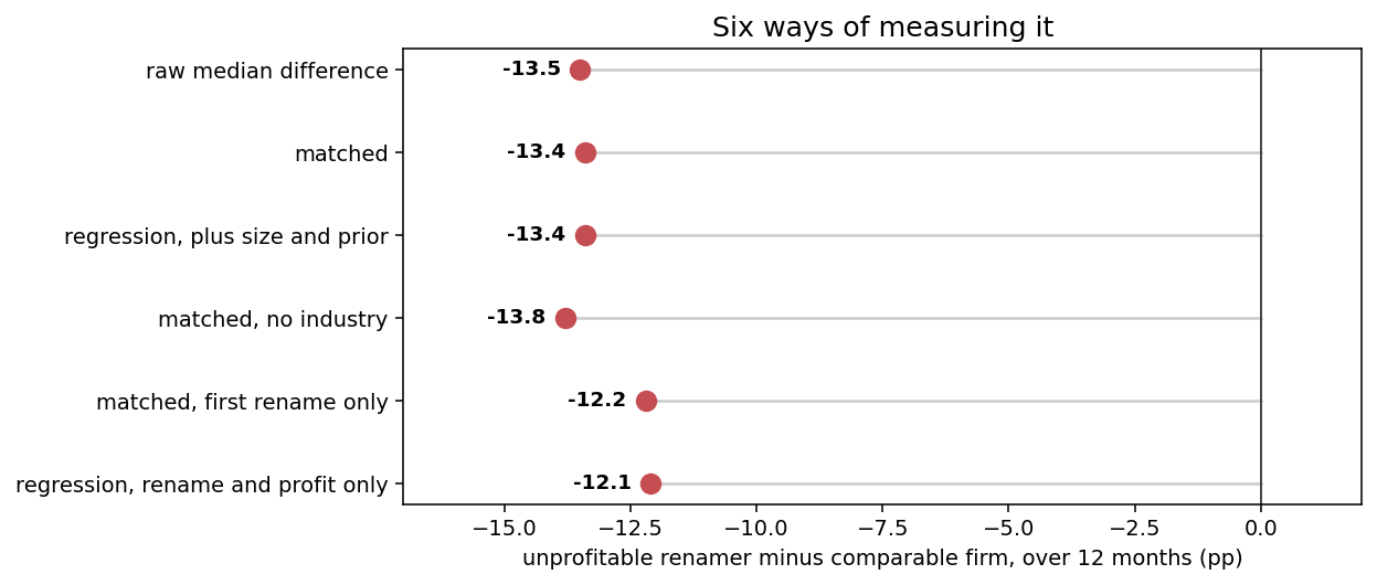
All six estimates are negative and of similar size, so the result does not rest on one way of measuring it. Nominal 95% intervals, from rerunning the matching on random subsets of the firms, are below zero at all three subset sizes, and the paired difference is negative for 200 of the 332 unprofitable renaming firms (Appendix B).
The same comparison in calendar time
The twelve-month windows overlap: renames one month apart share eleven months of returns, so treating them as independent may overstate the result’s precision (Mitchell and Stafford, 2000). In calendar time, each month \(\tau\) gets one number, the average over the unprofitable renames active that month of the renamer’s return minus its matched controls’ average return,
\[S_\tau = \frac{1}{N_\tau}\sum_{i \in E_\tau}\Big(r_{i,\tau} - \frac{1}{K_{i,\tau}}\sum_{j \in C_{i,\tau}} r_{j,\tau}\Big),\]
where \(E_\tau\) holds the \(N_\tau\) unprofitable renames for which \(\tau\) is one of the twelve months after the rename and which traded in \(\tau\) along with at least one matched control, and \(C_{i,\tau}\) holds the \(K_{i,\tau}\) matched controls of rename \(i\) that traded in \(\tau\). A regression of \(S_\tau\) on a constant estimates its mean and tests whether that mean is zero.
# The matched pairs of the unprofitable renamers, and every firm's monthly returns
unprofitable_pairs = pairs[pairs['Unprof'] == 1]
returns = monthly_panel[['Instrument', 'ym', 'ret']]

# Each pair once for each of the twelve months after the rename
pieces = []
for month_ahead in range(1, HORIZON + 1):
    step = unprofitable_pairs[['event', 'Instrument', 'Instrument_c', 'ym']].copy()
    step['ym'] = step['ym'] + month_ahead          # a Period plus k is k months later
    pieces.append(step)
steps = pd.concat(pieces, ignore_index=True)

# The renamer's and the control's return that month; a pair counts only if both traded
firm_returns = returns.rename(columns={'ret': 'r_firm'})
control_returns = returns.rename(columns={'Instrument': 'Instrument_c', 'ret': 'r_ctrl'})
steps = steps.merge(firm_returns, on=['Instrument', 'ym'], how='left')
steps = steps.merge(control_returns, on=['Instrument_c', 'ym'], how='left')
steps = steps.dropna(subset=['r_firm', 'r_ctrl'])

# Per event and month: the renamer's return minus its controls' average
by_event_month = steps.groupby(['event', 'ym'])
event_months = pd.DataFrame({'r_firm': by_event_month['r_firm'].first(),
                             'r_ctrl': by_event_month['r_ctrl'].mean()}).reset_index()
event_months['spread'] = event_months['r_firm'] - event_months['r_ctrl']

# S_tau: the average over the events active in each calendar month
monthly_spread = event_months.groupby('ym')['spread'].mean().sort_index()

# A regression on a constant alone estimates the mean and tests whether it is zero
spread_values = monthly_spread.values
constant = np.ones((len(spread_values), 1))

active_events = event_months.groupby('ym').size().median()      # events per month, median
print(f'{len(spread_values)} months, median {active_events:.0f} active events, '
      f'mean monthly difference {spread_values.mean() * 100:+.2f}%')

for lags in (0, 6, 12):
    if lags == 0:
        fitted = sm.OLS(spread_values, constant).fit()          # ordinary standard errors
    else:
        # Newey-West standard errors allow nearby months to be correlated
        fitted = sm.OLS(spread_values, constant).fit(cov_type='HAC',
                                                     cov_kwds={'maxlags': lags})
    print(f'  Newey-West {lags:>2}: t = {fitted.tvalues[0]:>6.2f}  p = {fitted.pvalues[0]:.4f}')
300 months, median 12 active events, mean monthly difference -0.57%
Newey-West 0: t = -1.44 p = 0.1502
Newey-West 6: t = -1.52 p = 0.1292
Newey-West 12: t = -1.40 p = 0.1614The line labelled 0 uses ordinary standard errors, and the other two use Newey-West standard errors with 6 and 12 lags, which allow nearby months to be correlated. With all three, the mean monthly difference is not statistically different from zero at the 5% level, so in calendar time the difference is too imprecise to distinguish from zero.
Limitations
Matching balances what I can measure. Distress that I cannot measure may explain both the rename and the return that follows. So a rename by an unprofitable firm predicts a lower return, and the design does not show that the rename causes it.
The difference is not a trading strategy. A difference between two groups’ returns is not the return of a portfolio until we say how it is financed, and in calendar time the difference is not distinguishable from zero.
The sample needs all twelve months. Firms that leave the panel inside the window cannot enter, and the data does not say whether a firm delisted after failing or after an acquisition, so the direction of this bias is unknown.
Appendix A lists the limits of the data itself.
Conclusion
The takeaway is that a name change on its own was no signal to sell: the underperformance after renaming was concentrated among firms that were already unprofitable. The data does not record why a struggling firm renames. A rename may be a real change of business, and it may be an attempt to leave a reputation behind. Both look the same in a returns panel.
Appendix
The code runs in this order: Appendix A builds the sample, the blocks in the main text compute the results, and Appendix B runs the additional checks. It needs the licensed data, so it does not run on this page, and with the same data it reproduces every number.
A. Building the sample
The data come from LSEG: a daily panel of US stock returns and market values, annual accounts with the dates they were announced, the S&P 500 total-return index (dividends reinvested), industry groups, and the identifiers that link a company across its names. Because the data is licensed, I cannot share the raw files.
LSEG’s search index holds each company’s earlier names with the dates they were valid, including companies that have since delisted, which matters because many of the distressed firms in this study no longer trade. It gives 8,985 rename records from 5,369 companies.
Many records change only the capitalisation, the punctuation or the legal form, such as Corp to Inc, and I drop them. I also remove special-purpose acquisition companies (SPACs), which are shells set up to buy another firm, as well as funds, firms domiciled outside the US, and renames that coincide with a deal. Say company A buys company B, doubles its revenue and renames, and the stock rises. Attributing that to the name would be wrong, so any rename within twelve months of a deal event goes. A rename can be measured only if the stock traded that month, and 1,955 renames pass every filter. A.4 counts each exclusion.
The code expects five inputs.
- The daily panel on disk, one row per stock-day:
Instrument,Date,Daily Total Return,Company Market Cap,Deal Event Announcement Date,Deal Event Type. It is read once, in chunks. f, one row per firm-year of accounts:Instrument,announce_date,net_income,assets. Using the announcement date means the profitability measure contains only information that was public at the time.spx, monthly levels of the S&P 500 total-return index.SPXTR, with columnsymandlevel. The stock returns are total returns, so the benchmark has to be one too, and.SPXis price-only.static, one row per firm:Instrumentandindustry, the TRBC industry group name.ric_map, one row per ticker:InstrumentandOrgPermID. I use it to link the same company before and after a name change.
Throughout, ym is a monthly period and every return is a decimal.
import re                            # cleaning up company names
import difflib                       # how similar two strings are
import numpy as np
import pandas as pd
import statsmodels.api as sm         # regressions with clustered standard errors
import matplotlib.pyplot as plt
from scipy import stats              # the binomial test behind the sign test

PANEL   = r'US_stocks.csv'   # the daily panel, 27.4M rows
HORIZON = 12                 # months on each side of the event
BUFFER  = 24                 # exclude the 24 months before a firm's first rename
N_MATCH = 5                  # controls per renamer
CALIPER = 0.60               # maximum standardised distance to a control
RED, BLUE, GREY = '#C44E52', '#1F77B4', '#CCCCCC'LSEG does not expose historical names through the usual TR.* fields. TR.CompanyName returns today’s name even when given a past date. I found the historical names in the search index, in the ORGANISATIONS view, under a property called PreviousNames.
import lseg.data as ld

ld.get_config().set_param('http.request-timeout', 300)   # raise this BEFORE open_session
ld.open_session()

df = ld.discovery.search(
    view=ld.discovery.Views.ORGANISATIONS,
    filter="OAPermID in ('4295905573')",                 # space-separated inside in(...)
    select='CommonName,LegalName,PreviousNames,OAPermID,OrganisationStatus',
)
I lost an afternoon to two syntax details. The select string has to be comma-separated; a semicolon returns zero rows without an error. The values inside in (...) have to be space-separated, while a comma raises Invalid filter: found COMMA in IN_CLAUSE.
I use the organisation PermID, LSEG’s permanent identifier for a company, as the join key because it does not change when a firm changes its name or ticker, or when it delists. I pull the 10,078 tickers in my US panel in batches of 100 and map each one to its PermID with TR.OrganizationID. I then query the search index for that organisation’s history and combine the batches into one frame, org, with one row per organisation.
PreviousNames comes back as a flat list of [old name, valid from, valid to], newest first, with consecutive records glued together by a tilde. A made-up record for a firm renamed once looks like ['Old Name, Inc.', '1995-03-01', '2004-06-30'].
def parse_previous_names(cell):
    """One PreviousNames cell into a list of (old_name, valid_from, valid_to), newest first."""
    if not isinstance(cell, (list, np.ndarray)) or len(cell) == 0:
        return []

    # The list holds the fields of every record in one flat row, with the tilde
    # inside the field where one record ends and the next begins. Joining the fields with
    # NUL, a character no company name contains, gives one string that can be split on the
    # tilde first and on the field boundaries second.
    text = '\x00'.join(str(x) for x in cell)

    records = []
    for record in text.split('~'):
        parts = record.split('\x00')
        if len(parts) >= 3 and parts[0].strip():
            records.append((parts[0].strip(), parts[1].strip(), parts[2].strip()))
    return records


rows = []
for _, row in org.iterrows():
    records = parse_previous_names(row.get('PreviousNames'))
    current = row.get('LegalName') or row.get('CommonName')

    for i, (old_name, valid_from, valid_to) in enumerate(records):
        # Records arrive newest first, so the name that replaced record i is record i-1,
        # and the newest old name was replaced by the name the company uses today.
        new_name = current if i == 0 else records[i - 1][0]

        rows.append({'OrgPermID': row.get('OAPermID'),
                     'OldName': old_name,
                     'NewName': new_name,
                     'ValidFrom': valid_from,
                     'RenameDate': valid_to,          # the day the old name stopped being valid
                     'Status': row.get('OrganisationStatus'),
                     'Country': row.get('CountryHeadquartersName')})

renames = pd.DataFrame(rows)

# errors='coerce' turns an unreadable date into NaT instead of stopping the run
renames['RenameDate'] = pd.to_datetime(renames['RenameDate'], errors='coerce')
print(f'{len(renames):,} rename records from {renames["OrgPermID"].nunique():,} companies')
8,985 rename records from 5,369 companiesThe same call returns OrganisationStatus, which marks the organisations that have delisted.
I first compound daily returns into monthly returns. In the same pass, I store the deal events used by the deal filter in A.4. Log returns are additive, so a month split across two chunks of a 2.7 GB file can be summed back together at the end.
USE = ['Instrument', 'Date', 'Daily Total Return', 'Company Market Cap',
       'Deal Event Announcement Date', 'Deal Event Type']

monthly_parts, mcap_parts, deal_parts = [], [], []

# The file is too large to hold at once, so pandas hands it over a million rows at a time.
# Each chunk is reduced to three small tables, and the pieces are combined afterwards.
for chunk in pd.read_csv(PANEL, chunksize=1_000_000, usecols=USE, low_memory=False):
    chunk['Date'] = pd.to_datetime(chunk['Date'], errors='coerce')
    chunk = chunk.dropna(subset=['Date', 'Instrument'])

    # A Period names the month, so every day of March 2007 groups together as 2007-03
    chunk['ym'] = chunk['Date'].dt.to_period('M')

    # Deal announcements are rare rows in the panel. Only those are kept, for the deal filter in A.4.
    deals_here = chunk.dropna(subset=['Deal Event Announcement Date'])
    deal_parts.append(deals_here[['Instrument', 'Deal Event Announcement Date',
                                  'Deal Event Type']].drop_duplicates())

    # Log returns add up over days. log1p(r) is log(1 + r), so a
    # month's returns can be summed inside this chunk now and across chunks below.
    daily_return = pd.to_numeric(chunk['Daily Total Return'], errors='coerce') / 100.0

    # Cap at plus and minus 100%: the raw file has returns up to +89,900% in a day on corrupted rows
    daily_return = daily_return.clip(-1.0, 1.0)
    chunk['logret'] = np.log1p(daily_return)

    # groupby.sum() already skips a missing day. Dropping those rows first also drops a
    # month whose days are all missing, which would otherwise arrive as a zero return.
    has_return = chunk.dropna(subset=['logret'])
    monthly_parts.append(
        has_return.groupby(['Instrument', 'ym'], observed=True)['logret'].sum())

    # The latest market cap observed in the month. Sorting by date first makes last() the
    # latest observation rather than whichever row the file happened to list last.
    caps = chunk.dropna(subset=['Company Market Cap']).sort_values('Date')
    mcap_parts.append(
        caps.groupby(['Instrument', 'ym'], observed=True)[['Company Market Cap', 'Date']].last())

# A month that straddles two chunks now has two partial sums. Grouping again adds them.
monthly = pd.concat(monthly_parts).reset_index()
monthly = monthly.groupby(['Instrument', 'ym'])['logret'].sum().reset_index()
monthly['ret'] = np.expm1(monthly['logret'])       # expm1 undoes log1p: back to a simple return

# The same month can also have a market cap from each chunk. The later date wins.
mcap = pd.concat(mcap_parts).reset_index().sort_values('Date')
mcap = mcap.groupby(['Instrument', 'ym']).last().reset_index()
mcap = mcap[['Instrument', 'ym', 'Company Market Cap']]

# how='left': a month without a market cap still keeps its return
monthly_panel = monthly[['Instrument', 'ym', 'ret']].merge(
    mcap, on=['Instrument', 'ym'], how='left')

print(f'{len(monthly_panel):,} firm-months across '
      f'{monthly_panel["Instrument"].nunique():,} firms')
1,348,652 firm-months across 10,064 firmsThe daily file compounds into 1,348,652 firm-months across 10,064 firms. I put every firm on a continuous monthly grid, so a gap in trading is a missing month and eleven traded months never count as a year. The main text calculates the adjusted returns on that grid.
# Every firm goes on a continuous monthly grid, so that twelve rows are always twelve
# calendar months. A month with no trading becomes a missing row rather than vanishing,
# which would otherwise let eleven traded months pass as a year.
span = monthly_panel.groupby('Instrument')['ym'].agg(['min', 'max'])

pieces = []
for firm, row in span.iterrows():
    months = pd.period_range(row['min'], row['max'], freq='M')
    pieces.append(pd.DataFrame({'Instrument': firm, 'ym': months}))
grid = pd.concat(pieces, ignore_index=True)

# how='left': the grid decides which rows exist, the panel only fills them in
panel = grid.merge(monthly_panel, on=['Instrument', 'ym'], how='left')

spx['spx_lr'] = np.log1p(spx['level'].pct_change())
panel = panel.merge(spx[['ym', 'spx_lr']], on='ym', how='left')
panel = panel.merge(static[['Instrument', 'industry']], on='Instrument', how='left')

print(f'panel rows {len(panel):,}')
panel rows 1,350,926The grid has 1,350,926 rows, 2,274 more than the firm-months with trading, one for each month without trading.
The first block drops records whose name changes only in capitalisation, punctuation or legal form: it strips the legal-form words from both names and compares what is left.
LEGAL_WORDS = {'INC', 'INCORPORATED', 'CORP', 'CORPORATION', 'CO', 'COMPANY', 'LLC', 'LP',
               'LTD', 'LIMITED', 'PLC', 'SA', 'AG', 'NV', 'HOLDING', 'HOLDINGS', 'GROUP', 'THE'}


def normalise(name):
    """'Apple, Inc.' -> 'APPLE INC'. Case and punctuation are not a rename."""
    letters_only = re.sub(r'[^A-Z0-9 ]+', ' ', str(name).upper())
    return re.sub(r'\s+', ' ', letters_only).strip()     # runs of spaces become one


def core(name):
    """'APPLE INC' -> 'APPLE'. The business identity without its legal wrapper."""
    return ' '.join(word for word in normalise(name).split() if word not in LEGAL_WORDS)


def distance(old, new):
    """0 for identical names, 1 for names with nothing in common."""
    return 1 - difflib.SequenceMatcher(None, old, new).ratio()


# apply() runs a function on every value of a column and returns the results as a column
renames['OldCore'] = renames['OldName'].apply(core)
renames['NewCore'] = renames['NewName'].apply(core)

# Two comparisons sort the records into three kinds: only capitalisation or punctuation
# moved, only the legal wrapper moved ("X Corp" became "X Inc"), or the identity changed.
renames['CosmeticOnly'] = (renames['OldName'].apply(normalise)
                           == renames['NewName'].apply(normalise))
renames['LegalFormOnly'] = ((renames['OldCore'] == renames['NewCore'])
                            & ~renames['CosmeticOnly'])
renames['UseInStudy'] = ~renames['CosmeticOnly'] & ~renames['LegalFormOnly']

# When a firm renames twice in one month the next block keeps the larger change, so each
# record needs a size for that comparison.
renames['NameDistance'] = [distance(old, new)
                           for old, new in zip(renames['OldCore'], renames['NewCore'])]

# One organisation can have several tickers in the panel. A left merge gives each ticker
# its own event row, and an organisation with no ticker gets a missing one and drops out.
renames = renames.merge(ric_map[['Instrument', 'OrgPermID']], on='OrgPermID', how='left')
renames = renames.rename(columns={'Instrument': 'PanelRIC'})
renames['InPanelWindow'] = renames['RenameDate'].between('2000-01-01', '2026-02-27')
The second block removes SPACs, funds, foreign firms and renames within twelve months of a deal.
deals = pd.concat(deal_parts).drop_duplicates()
deals['DealDate'] = pd.to_datetime(deals['Deal Event Announcement Date'], errors='coerce')
deals = deals.dropna(subset=['DealDate'])

# A SPAC's old name is the shell, "XYZ Acquisition Corp II", and after the deal it takes
# the target's name, so only the old name is tested. Funds and trusts are not operating
# companies under either name.
SPAC_PAT = (r'\b(?:ACQUISITION|BLANK CHECK)\b'
            r'|\b(?:CAPITAL|HOLDINGS?)\s+(?:CORP|CORPORATION|CO)\b\s*'
            r'(?:I{1,3}|IV|V|VI{1,3}|IX|X{1,3}|\d+)?\s*$')   # sponsors run numbered series
FUND_PAT = r'\b(?:FUND|TRUST|ETF|PORTFOLIO|INDEX|REIT)\b'

OLD = renames['OldName'].fillna('').str.upper()
NEW = renames['NewName'].fillna('').str.upper()

renames['IsSPAC'] = OLD.str.contains(SPAC_PAT, regex=True, na=False)
renames['IsFund'] = OLD.str.contains(FUND_PAT, na=False) | NEW.str.contains(FUND_PAT, na=False)
renames['IsForeign'] = renames['Country'].notna() & (renames['Country'] != 'United States')

renames['PureRename'] = (renames['UseInStudy'] & renames['InPanelWindow']
                         & ~renames['IsSPAC'] & ~renames['IsFund'] & ~renames['IsForeign'])

# A list of deal dates per ticker, so each rename is checked against a few dates rather
# than against the whole deal table.
deal_dates = deals.groupby('Instrument')['DealDate'].apply(list)


def near_deal(ticker, when):
    """Any deal announced within twelve months either side of the rename?"""
    if pd.isna(when) or ticker not in deal_dates.index:
        return False
    # DateOffset counts calendar months, so the window ends on the same day of the month
    earliest = when - pd.DateOffset(months=HORIZON)
    latest = when + pd.DateOffset(months=HORIZON)
    return any(earliest <= date <= latest for date in deal_dates[ticker])


renames['NearDeal'] = [near_deal(ticker, when)
                       for ticker, when in zip(renames['PanelRIC'], renames['RenameDate'])]
renames['PureRenameNoDeal'] = renames['PureRename'] & ~renames['NearDeal']
I count the exclusions in the order I apply them. The last filter uses the monthly panel from A.3.
# Each filter applies after the ones before it. The count after each is kept for the table.
funnel = []
funnel.append(('Raw name records, joined to panel tickers', len(renames)))
funnel.append(('Not cosmetic, not legal-form only', int(renames['UseInStudy'].sum())))
funnel.append(('Rename date inside the 2000-2026 panel',
               int((renames['UseInStudy'] & renames['InPanelWindow']).sum())))
funnel.append(('Not a SPAC, fund or foreign domicile', int(renames['PureRename'].sum())))
funnel.append(('No deal event within twelve months', int(renames['PureRenameNoDeal'].sum())))

# copy(): a table of its own, so the columns added below leave `renames` untouched
rename_events = renames[renames['PureRenameNoDeal'] & renames['PanelRIC'].notna()].copy()
rename_events['ym'] = rename_events['RenameDate'].dt.to_period('M')

# drop_duplicates keeps the first row it meets, so sorting by NameDistance first keeps the
# largest change when a firm renames twice in the same month.
rename_events = (rename_events.sort_values('NameDistance', ascending=False)
                              .drop_duplicates(['PanelRIC', 'ym'])
                              .rename(columns={'PanelRIC': 'Instrument'})
                              .sort_values('RenameDate'))
funnel.append(('One event per firm-month', len(rename_events)))

# A rename can only be measured if the stock traded that month. A left merge with
# indicator=True adds a column saying whether each event found its firm-month in the
# monthly panel: 'both' if it did, 'left_only' if not.
traded = monthly_panel[['Instrument', 'ym']]
found = rename_events.merge(traded, on=['Instrument', 'ym'],
                            how='left', indicator=True)['_merge']

# to_numpy(), because the merge result has new row labels
keep = (found == 'both').to_numpy()
dropped, rename_events = rename_events[~keep], rename_events[keep]
funnel.append(('Trading in the rename month', len(rename_events)))

funnel_table = pd.DataFrame(funnel, columns=['restriction', 'events'])

# shift(1) puts the previous count beside each row. Int64 is an integer column that allows
# the missing value in the first row.
funnel_table['lost'] = (funnel_table['events'].shift(1)
                        - funnel_table['events']).astype('Int64')
print(funnel_table.to_string(index=False))| Restriction | Events | Lost |
|---|---|---|
| Raw name records, joined to panel tickers | 8,990 | |
| Not cosmetic, not legal-form only | 7,990 | 1,000 |
| Rename date inside the 2000-2026 panel | 5,690 | 2,300 |
| Not a SPAC, fund or foreign domicile | 4,293 | 1,397 |
| No deal event within twelve months | 4,177 | 116 |
| One event per firm-month | 4,096 | 81 |
| Trading in the rename month | 1,955 | 2,141 |
The first row is larger than the 8,985 records parsed because one organisation may have several tickers in the panel. The join gives each ticker its own row.
The last filter removes 2,141 events. I check whether each one is before, during or after the firm’s time in the panel. I also count how many of the 5,690 records inside the sample window belong to companies that have since delisted.
# Was each dropped event before the firm's first traded month, after its last, or between?
where = []
for firm, month in zip(dropped['Instrument'], dropped['ym']):
    if firm not in span.index:                  # a ticker the price panel never saw at all
        continue
    if month < span.loc[firm, 'min']:
        where.append('before the firm appears')
    elif month > span.loc[firm, 'max']:
        where.append('after the firm leaves')
    else:
        where.append('inside the span')
print(pd.Series(where).value_counts().to_dict())

in_window = renames['UseInStudy'] & renames['InPanelWindow']
delisted = int((in_window & (renames['Status'] == 'Delisted')).sum())
print(f'delisted rename records inside the panel window: {delisted:,} of {int(in_window.sum()):,}')
{'before the firm appears': 1443, 'after the firm leaves': 693, 'inside the span': 5}
delisted rename records inside the panel window: 2,948 of 5,690So, 1,443 of the dropped events happen before the company enters the panel and 693 after it leaves, and neither has a stock return to measure. Only 5 are inside a firm’s time in the panel.
Of the 5,690 records inside the sample window, 2,948 belong to organisations marked as delisted. A sample built from tickers that trade today would miss over half of them, which is why I take the names from the search index, where delisted organisations remain.
I screen deal-driven renames with code. Wu (2010) reads press releases and filings by hand. My filter flagged 116 events as deal-related, but the code may have missed some. This is the main place where my method is weaker than Wu’s.
My date is the effective date. That is the day the old legal name stopped being valid. The announcement is sometimes on the same day and sometimes a year earlier, so these dates cannot support a clean short-window announcement study. Hand-collected announcement dates could.
I only have the current industry classification. I match firms on the industry group they have today. A company that changed business before changing its name may have received that label only later. Dropping the industry requirement entirely gives -13.8 percentage points.
I clean the daily returns before compounding. The raw file has corrupted values up to +89,900% in a single day, so I first cap daily total returns at plus and minus 100%.
B. Additional checks
These checks run after the main text’s code. Each one tests a part of the comparison: the result before matching, regressions, the balance of the matched firms, six estimates of the unprofitable renamers’ difference, and the uncertainty of the matched estimate.
Before matching, I compare every renamer with every eligible control. Table B1 gives the twelve-month adjusted return for all firms (Panel A) and by profitability before the rename (Panel B).
def summary(renamers, others):
    """Table B1: renamers against controls on the 12-month adjusted return, in percent."""
    renamer_returns = renamers['ER_post12']
    control_returns = others['ER_post12']

    print(f'{len(renamer_returns):,} renamer events from '
          f'{renamers["Instrument"].nunique():,} firms, '
          f'{len(control_returns):,} control firm-months from '
          f'{others["Instrument"].nunique():,} firms')

    table = pd.DataFrame(
        {'Renamers': [renamer_returns.mean(), renamer_returns.median(),
                      (renamer_returns < 0).mean()],
         'Controls': [control_returns.mean(), control_returns.median(),
                      (control_returns < 0).mean()]},
        index=['Mean adjusted return', 'Median adjusted return',
               'Share below the S&P 500']) * 100

    table['Difference'] = table['Renamers'] - table['Controls']
    return table.round(1)


print(summary(treated, controls).to_string())
This block prints Table B1, Panel A.
Table B1, Panel A. All firms. 12-month S&P 500-adjusted total return.
| Renamers | Eligible controls | Difference | |
|---|---|---|---|
| Observations | 1,571 | 971,060 | |
| Firms | 1,346 | 8,099 | |
| Mean adjusted return | 0.8% | 4.5% | -3.6pp |
| Median adjusted return | -7.6% | -2.5% | -5.1pp |
| Share below the S&P 500 | 56.7% | 53.8% | +2.9pp |
The median adjusted return of the renamers is 5.1 percentage points below that of the controls, and the mean is 3.6 points below. The two differ because twelve-month returns are strongly right-skewed: a few very large returns increase the mean. I compare groups by their medians, which describe the typical firm.
I leave test statistics out of this table. The 1,571 renamers are compared with about a million control firm-months whose twelve-month windows overlap heavily, and a two-sample t-test would treat those control observations as independent when they are not.
The 5.1 points could come from renaming or from the kind of firm that renames. I split the events by whether the firm was profitable before the rename, and label each control the same way, with the accounts known at the start of its month.
# A control is labelled the way a renamer is, with the accounts known at the start of its month
all_rows = pd.concat([treated, controls], ignore_index=True)
month_start = all_rows['ym'].dt.to_timestamp()          # a Period to the first day of its month
net_income = latest_accounts(all_rows['Instrument'], month_start)['net_income']
all_rows['Unprof_ms'] = np.where(net_income.notna(),
                                 (net_income < 0).astype(float), np.nan)

# The rows that have a label. The regressions in B.2 run on these.
labelled = all_rows.dropna(subset=['Unprof_ms']).copy()

labelled_controls = labelled[labelled['Rename'] == 0]
print(f'controls carrying a month-start label: {len(labelled_controls):,}')

profitable_renamers = treated[treated['Unprof'] == 0]
profitable_controls = labelled_controls[labelled_controls['Unprof_ms'] == 0]
unprofitable_renamers = treated[treated['Unprof'] == 1]
unprofitable_controls = labelled_controls[labelled_controls['Unprof_ms'] == 1]

print(summary(profitable_renamers, profitable_controls).to_string())
print(summary(unprofitable_renamers, unprofitable_controls).to_string())

# Kept for the six estimates in B.4
unprof_renamer_returns = unprofitable_renamers['ER_post12']
unprof_control_returns = unprofitable_controls['ER_post12']

print(f'unprofitable renamers above +100%: '
      f'{(unprof_renamer_returns > 1.0).mean() * 100:.1f}%, '
      f'max {unprof_renamer_returns.max() * 100:+.0f}%')
This block prints Table B1, Panel B, and the share of unprofitable renamers above +100%. Among unprofitable renamers, 7.9% had a 12-month adjusted return above +100 percentage points, and the highest was +754 percentage points. With those few large adjusted returns included, the mean is -5.4%, far above the median of -22.6%.
Table B1, Panel B. By profitability before the rename. I measure profitability at month start for 787,268 controls.
| Prof. renamer | Controls | Diff. | Unprof. renamer | Controls | Diff. | |
|---|---|---|---|---|---|---|
| Observations | 926 | 571,934 | 645 | 215,334 | ||
| Mean adjusted return | 5.2% | 4.2% | +0.9pp | -5.4% | 7.3% | -12.7pp |
| Median adjusted return | -0.4% | -1.2% | +0.8pp | -22.6% | -9.0% | -13.5pp |
| Share below the S&P 500 | 50.1% | 51.8% | -1.7pp | 66.0% | 58.3% | +7.7pp |
Among profitable firms, the median difference is +0.8 percentage points. Among unprofitable firms it is -13.5. Panel A, which pools both groups, gives -5.1, so almost all of that difference comes from the unprofitable firms.
In the regression every firm, renamer or control, is labelled with the accounts known at the start of its month. I subtract each calendar month’s average from every variable, which removes anything common to all firms in that month, such as the market’s return. These are calendar-month fixed effects. The standard errors are clustered by firm and by calendar month, which allows the returns of one firm, and of one month, to be correlated.
# The interaction: 1 only for an unprofitable renamer
labelled['RxU'] = labelled['Rename'] * labelled['Unprof_ms']


def twoway(table, outcome, predictors):
    """OLS with calendar-month fixed effects, clustered by firm and by month."""
    demeaned = table.dropna(subset=[outcome] + predictors).copy()

    # Subtracting each month's mean from every variable is the same as adding a dummy for
    # every month, and it keeps the design matrix at a handful of columns.
    for column in [outcome] + predictors:
        demeaned[column] = (demeaned[column]
                            - demeaned.groupby('ym', observed=True)[column].transform('mean'))

    # statsmodels wants each cluster as an integer code, one column per clustering dimension
    firm_id = pd.factorize(demeaned['Instrument'])[0]
    month_id = pd.factorize(demeaned['ym'])[0]
    groups = np.column_stack([firm_id, month_id])

    fitted = sm.OLS(demeaned[outcome], sm.add_constant(demeaned[predictors])).fit(
        cov_type='cluster', cov_kwds={'groups': groups})
    return fitted, len(demeaned)


SPECS = {'(1)': ['Rename'],
         '(2)': ['Rename', 'Unprof_ms', 'RxU'],
         '(3)': ['Rename', 'Unprof_ms', 'RxU', 'ER_pre12', 'log_mcap']}

models = {column: twoway(labelled, 'ER_post12', predictors)
          for column, predictors in SPECS.items()}


def stars(p_value):
    """The significance marks the table caption describes: 0.10, 0.05 and 0.01."""
    if p_value < 0.01:
        return '***'
    if p_value < 0.05:
        return '**'
    if p_value < 0.10:
        return '*'
    return ''


# The table is printed by hand rather than by pandas, because each variable takes two
# lines: the coefficient with its stars, and the t-statistic in parentheses underneath.
VARIABLES = ['Rename', 'Unprof_ms', 'RxU', 'ER_pre12', 'log_mcap']
WIDTH = 13                                    # characters per specification column

print(f'{"":<12}' + ''.join(f'{column:>{WIDTH}}' for column in SPECS))

for variable in VARIABLES:
    coefficient_line = f'{variable:<12}'
    t_statistic_line = ' ' * 12

    for column in SPECS:
        model = models[column][0]
        if variable in model.params.index:
            coefficient = f'{model.params[variable]:+.4f}{stars(model.pvalues[variable]):<3}'
            coefficient_line += coefficient.rjust(WIDTH)
            t_statistic_line += f'({model.tvalues[variable]:.2f})'.rjust(WIDTH)
        else:
            coefficient_line += ' ' * WIDTH    # this variable is not in this specification
            t_statistic_line += ' ' * WIDTH

    print(coefficient_line)
    print(t_statistic_line)

print(f'{"N":<12}' + ''.join(f'{models[column][1]:>{WIDTH},}' for column in SPECS))
Table B2. Regressions. t-statistics, each estimate divided by its standard error, in parentheses. Stars mark p-values below 0.10, 0.05 and 0.01, where a p-value is the chance of an estimate this far from zero if the true value were zero. Coefficients are in decimal-return units, so -0.121 is -12.1 percentage points.
| (1) | (2) | (3) | |
|---|---|---|---|
| Rename | -0.031 | +0.013 | +0.002 |
| (-1.60) | (0.80) | (0.14) | |
| Unprofitable | +0.045*** | +0.040*** | |
| (3.11) | (3.16) | ||
| Rename × Unprofitable | -0.121*** | -0.134*** | |
| (-2.97) | (-3.14) | ||
| Prior 12-month adjusted return | -0.021*** | ||
| (-3.10) | |||
| Log market cap | -0.015*** | ||
| (-5.90) | |||
| Observations | 788,823 | 788,823 | 722,680 |
Column (1) pools all firms. The rename coefficient is -3.1 percentage points with a t-statistic of -1.60, not statistically different from zero at the 10% level. It is the regression version of Table B1, Panel A, and like every coefficient here it estimates a difference in means.
Column (2) separates profitable and unprofitable firms. The Rename coefficient is the estimate for profitable renamers, +1.3 percentage points. For an unprofitable renamer the interaction, Rename × Unprofitable, is added, so the estimate is \(1.3-12.1=-10.8\) percentage points.
Column (3) adds the prior twelve-month adjusted return and log market cap. The same sum gives \(0.2-13.4=-13.2\) percentage points for unprofitable renamers.
I check whether the matched firms were similar to the unprofitable renamers on size, prior return and return on assets. A standardised difference is the renamers’ average minus the matched firms’ average, divided by the pooled standard deviation, so 0 means equal averages.
def standardised_difference(renamer_values, control_values):
    """The difference between two groups, measured in pooled standard deviations."""
    renamer_values, control_values = renamer_values.dropna(), control_values.dropna()
    pooled = np.sqrt((renamer_values.var(ddof=1) + control_values.var(ddof=1)) / 2)
    if pooled == 0:
        return np.nan
    return (renamer_values.mean() - control_values.mean()) / pooled


def standardised_difference_weighted(renamer_side, control_side, weights, covariate):
    """The same, with every control weighted by its share of its own matched set."""
    renamer_mean = renamer_side[covariate].mean()
    renamer_var = renamer_side[covariate].var(ddof=1)
    control_mean = np.average(control_side[covariate], weights=weights)
    control_var = np.average((control_side[covariate] - control_mean) ** 2, weights=weights)
    return (renamer_mean - control_mean) / np.sqrt((renamer_var + control_var) / 2)


# The balance table compares each unprofitable renamer with its own matched set. Every pair
# of an event repeats the renamer's covariates, so first() reads them once per event, and
# mean() over the _c columns gives that event's matched-set average.
renamer_covariates = unprofitable_pairs.groupby('event')[COVARIATES].first()
matched_set_means = unprofitable_pairs.groupby('event')[
    ['log_mcap_c', 'ER_pre12_c', 'roa_c']].mean()
matched_set_means.columns = COVARIATES        # the same names, so the two tables align

# One row per control, with its share of its matched set
each_control = unprofitable_pairs[['log_mcap_c', 'ER_pre12_c', 'roa_c', 'weight']].copy()
each_control.columns = COVARIATES + ['weight']

print(f'{"covariate":<12}{"set-mean":>12}{"share weighted":>16}')
for covariate in COVARIATES:
    set_mean = standardised_difference(renamer_covariates[covariate],
                                       matched_set_means[covariate])
    weighted = standardised_difference_weighted(renamer_covariates, each_control,
                                                each_control['weight'], covariate)
    print(f'{covariate:<12}{set_mean:>+12.3f}{weighted:>+16.3f}')
This block prints Table B3. The set-mean column compares each renamer with the average of its own matched set, and the share-weighted column weights each control by its share of its set. The two weightings agree to within 0.001.
Table B3. Balance after matching for unprofitable firms. Standardised mean differences.
| Covariate | Set-mean | Share weighted |
|---|---|---|
| Log market cap | -0.035 | -0.035 |
| Prior 12-month adjusted return | +0.017 | +0.016 |
| Return on assets | -0.011 | -0.011 |
All three standardised differences are smaller than 0.04 in absolute value under both weightings. The firms may still differ in ways I cannot observe.
Five other estimates of the same difference are the raw difference in medians from Table B1, two regressions (B.2), matching without the industry requirement, and matching on only each firm’s first rename among the events that pass the filters. A regression is a statistical fit of the return on the rename and other variables, and these two compare firms within the same calendar month. The four matched and raw estimates are medians, and the two regression estimates are differences in means.
This block computes the six estimates and draws the chart in the main text. It prints the six estimates, in percentage points: -13.5 for the raw difference in medians, -13.4 matched, -13.8 matched without the industry requirement, -12.2 matched on first renames only, and -10.8 and -13.2 for the two regressions, without and with size and prior return.
matched_unprofitable = matched_events[matched_events['Unprof'] == 1]

# The same matching without the industry requirement
matched_no_industry = match(treated, controls, use_industry=False)[0]
matched_no_industry = matched_no_industry[matched_no_industry['Unprof'] == 1]

# Only each firm's first rename among the events that passed the filters
first = treated.sort_values('ym').groupby('Instrument')['ym'].first()
matched_first_rename = matched_unprofitable[
    matched_unprofitable['ym'] == matched_unprofitable['firm'].map(first)]

# For an unprofitable firm the rename effect is the sum of the two coefficients
regression_full = (models['(3)'][0].params['Rename'] + models['(3)'][0].params['RxU']) * 100
regression_simple = (models['(2)'][0].params['Rename'] + models['(2)'][0].params['RxU']) * 100

SIX_WAYS = [('raw median difference',
         (unprof_renamer_returns.median() - unprof_control_returns.median()) * 100),
        ('matched', matched_unprofitable['diff'].median() * 100),
        ('regression, plus size and prior', regression_full),
        ('matched, no industry', matched_no_industry['diff'].median() * 100),
        ('matched, first rename only', matched_first_rename['diff'].median() * 100),
        ('regression, rename and profit only', regression_simple)]

for label, estimate in SIX_WAYS:
    print(f'{label:<36}{estimate:>+7.1f}pp')

fig, ax = plt.subplots(figsize=(9, 3.9))
for i, (label, estimate) in enumerate(SIX_WAYS):
    ax.plot([0, estimate], [i, i], color=GREY, lw=1.3, zorder=1)
    ax.plot(estimate, i, 'o', ms=9, color=RED, zorder=3)
    ax.annotate(f'{estimate:.1f}', (estimate, i), xytext=(-9, 0),
                textcoords='offset points', ha='right', va='center',
                fontsize=9.5, fontweight='bold')

ax.axvline(0, color='#444', lw=1.0)
ax.set_yticks(range(len(SIX_WAYS)))
ax.set_yticklabels([label for label, _ in SIX_WAYS], fontsize=10)
ax.invert_yaxis()
ax.set_xlabel('unprofitable renamer minus comparable firm, over 12 months (pp)')
ax.set_title('Six ways of measuring the unprofitable renamer difference', fontsize=13)
ax.set_xlim(-17, 2)
plt.tight_layout()
plt.savefig('nc_matched.png', dpi=140, bbox_inches='tight', facecolor='white')
raw median difference -13.5pp
matched -13.4pp
regression, plus size and prior -13.2pp
matched, no industry -13.8pp
matched, first rename only -12.2pp
regression, rename and profit only -10.8ppEach grey line starts at zero and ends at one estimate. The estimates range from about -10.8 to -13.8 percentage points. The three estimates without matching are close to the three estimates with matching.
The ordinary bootstrap puts an interval on an estimate by resampling the data with replacement and recomputing the estimate many times. Abadie and Imbens (2008) show that it can fail for nearest-neighbour matching, because a small change in the data can switch which controls are nearest. So, I use subsampling. Each draw takes a random subset of the renaming firms (treated in the code), without replacement, and the same proportion of the control firms, and runs the matching again from scratch, so the interval includes the uncertainty from choosing the partners. I run three subsample sizes, \(1{,}346^{0.6} \approx 75\), \(1{,}346^{0.7} \approx 155\) and \(1{,}346^{0.8} \approx 319\) of the 1,346 renaming firms, to show whether the interval depends on that choice.
treated_firms = treated['Instrument'].unique()
control_firms = controls['Instrument'].unique()
n_treated_firms, n_control_firms = len(treated_firms), len(control_firms)

full_sample_estimate = matched_unprofitable['diff'].median()
random_generator = np.random.default_rng(42)              # a fixed seed, so the intervals reproduce
intervals = []

for exponent in (0.60, 0.70, 0.80):
    # A subsample is much smaller than the sample and is drawn without replacement. Three
    # sizes are run to show whether the interval depends on that choice.
    draw_treated = int(round(n_treated_firms ** exponent))
    draw_controls = int(round(n_control_firms * draw_treated / n_treated_firms))

    draw_estimates = []
    for _ in range(400):
        picked_treated = set(random_generator.choice(
            treated_firms, size=draw_treated, replace=False))
        picked_controls = set(random_generator.choice(
            control_firms, size=draw_controls, replace=False))
        subsample_treated = treated[treated['Instrument'].isin(picked_treated)]
        subsample_controls = controls[controls['Instrument'].isin(picked_controls)]

        if len(subsample_treated) < 20 or len(subsample_controls) < 500:
            continue                          # a draw too small to match on is skipped

        # Matching runs again from scratch, so the interval includes the choice of partners
        draw_matched = match(subsample_treated, subsample_controls)[0]
        draw_unprofitable = draw_matched[draw_matched['Unprof'] == 1]
        if len(draw_unprofitable) > 5:
            draw_estimates.append(draw_unprofitable['diff'].median())

    # The subsampling root scales each draw's difference from the full-sample estimate by the
    # square root of the draw size. Its percentiles, scaled back by the square root of the
    # full sample, give the interval.
    scaled_gaps = np.sqrt(draw_treated) * (np.array(draw_estimates) - full_sample_estimate)
    # The upper percentile of the gaps gives the lower end of the interval, because each
    # end is the full-sample estimate minus a scaled gap.
    high_gap, low_gap = np.percentile(scaled_gaps, [97.5, 2.5])
    intervals.append((draw_treated,
                (full_sample_estimate - high_gap / np.sqrt(n_treated_firms)) * 100,
                (full_sample_estimate - low_gap / np.sqrt(n_treated_firms)) * 100))

    print(f'b=n^{exponent:.2f}: {draw_treated:>4} treated, {draw_controls:>5} controls, '
          f'95% [{intervals[-1][1]:+.1f}, {intervals[-1][2]:+.1f}]  ({len(draw_estimates)} draws)')

fig, ax = plt.subplots(figsize=(9, 3.9))
for i, (draw_treated, low, high) in enumerate(intervals):
    ax.plot([low, high], [i, i], color=BLUE, lw=3.0, solid_capstyle='round')
    ax.plot(full_sample_estimate * 100, i, 'o', ms=10, color=RED, zorder=3)
    ax.annotate(f'[{low:.1f}, {high:.1f}]', (low, i), xytext=(-8, 0),
                textcoords='offset points', ha='right', va='center',
                fontsize=10, fontweight='bold')

ax.axvline(0, color='#444', lw=1.4)
ax.set_yticks(range(len(intervals)))
ax.set_yticklabels([f'{draw} treated firms\nof {n_treated_firms:,}'
                    for draw, _, _ in intervals], fontsize=9.5)
ax.invert_yaxis()
ax.set_xlim(-40, 6)
ax.set_xlabel('95% interval for the unprofitable estimate (pp)')
ax.set_title('All three intervals are below zero', fontsize=13)
plt.tight_layout()
plt.savefig('nc_converge.png', dpi=140, bbox_inches='tight', facecolor='white')
b=n^0.60: 75 treated, 451 controls, 95% [-33.0, -4.0] (91 draws)
b=n^0.70: 155 treated, 933 controls, 95% [-27.1, -2.9] (395 draws)
b=n^0.80: 319 treated, 1919 controls, 95% [-24.1, -6.0] (400 draws)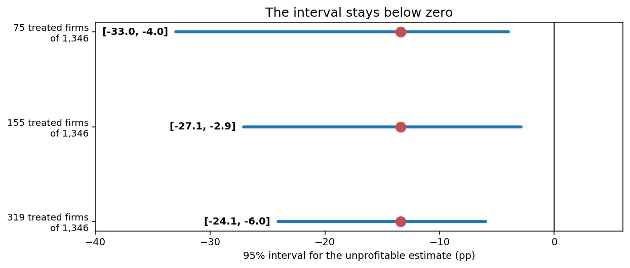
Each blue line is the nominal 95% interval at one subsample size. The red dot marks the full-sample estimate of -13.4. The intervals narrow as the subsample grows from 75 renaming firms to 319, and all three are below zero. At the largest size, the interval is -24.1 to -6.0 percentage points. The printed lines also give the renaming and control firms in each draw and how many of the 400 draws gave an estimate: at 155 renaming firms, the interval is -27.1 to -2.9, from 395 draws.
These intervals are nominal: the method aims at 95%, and nothing here shows that it achieves it. At the smallest size only 91 of the 400 draws had enough matched unprofitable events to give an estimate, so that interval rests on the draws where matching succeeded. Subsampling firms also leaves out shocks that hit many firms in the same month, which the calendar-time test in the main text allows for.
A sign test asks only whether the paired differences are negative more often than a coin toss would produce, so it makes no assumption about their size or distribution. I use one observation per firm, the median of its paired differences.
# One number per firm, so a firm that renamed twice still counts once
per_firm = matched_unprofitable.groupby('firm')['diff'].median()
negative, total = int((per_firm < 0).sum()), len(per_firm)

# The chance a fair coin gives a split at least this lopsided, in either direction
p_value = stats.binomtest(negative, total, 0.5).pvalue
print(f'{negative} of {total} negative, p = {p_value:.2e}')
200 of 332 negative, p = 2.25e-04The paired difference is negative for 200 of the 332 firms. If each firm’s sign were independent of the others’ and negative and positive were equally likely, a split at least this uneven, in either direction, would occur with a probability of 0.0002. That p-value is nominal, because firms share market movements and some share matched controls, so their signs are not fully independent.
C. Earlier studies
Kot (2011) studies Hong Kong renames and finds short-run price reactions but very little evidence of a long-run effect. My pooled result is also weak.
Wu (2010) finds that firms adopt a radically different name after their reputation has been tarnished, and that organisational upheaval follows most name changes. Guo and co-authors (2025) find that renaming predicts higher crash risk through diverted investor attention and greater information asymmetry. Their estimate is larger among firms with weak performance and poor governance. Both papers focus attention on firms already in trouble. In my data, the difference is also concentrated among firms that were unprofitable before the rename.
Andrikopoulos, Daynes and Pagas (2007) find a different pattern. Across 803 UK renames, they find long-run underperformance among firms with both positive and negative returns before the rename. In my data, profitable renamers show little: a median matched difference of -2.8 percentage points and a regression estimate of +0.2. They split firms by prior stock returns, and I split them by the income statement. Adding the prior twelve-month return to the regression does not remove my interaction, which is -12.1 percentage points without that control and -13.4 with it (Appendix B.2).
Read next
- Six biases that distort quant research, measured where the truth is known Six biases, each measured on a simulated market where the truth is known.
- Same data, same trading signal, different answer How much of a result comes from how the test was built.
- Download stock data from LSEG Workspace in Python The pipeline behind the panel used here.
Disclaimer: an empirical study for discussion purposes, not investment advice. The design is predictive and not causal. Past performance does not guarantee future returns.
Because the data is licensed, I cannot share the raw file, and every number above is an aggregate.
Sources: YiLin Wu, What’s in a name? What leads a firm to change its name and what the new name foreshadows, Journal of Banking & Finance 34(6), 1344-1359 (2010). Hung Wan Kot, Corporate name changes: Price reactions and long-run performance, Pacific-Basin Finance Journal 19(2), 230-244 (2011). Panagiotis Andrikopoulos, Arief Daynes and Paraskevas Pagas, The Long-Term Market Performance of UK Companies Following Corporate Name Changes, SSRN working paper (2007). Shijun Guo, Daifei Yao, Yefeng Zhang and Yuyu Zhang, Corporate Renaming and Stock Price Crash Risk, Accounting & Finance (2025). Alberto Abadie and Guido Imbens, On the Failure of the Bootstrap for Matching Estimators, Econometrica (2008). Mark Mitchell and Erik Stafford, Managerial Decisions and Long-Term Stock Price Performance, Journal of Business 73(3), 287-329 (2000).