Avoiding bad companies matters as much as finding great ones

A US backtest of the highest-quality companies against the lowest-quality, equal-weight and net of costs, 2000 to 2026. The best compounded; the worst fell 91%.

Avoiding bad companies matters as much as finding great ones. Buffett wrote that it is far better to buy a wonderful company at a fair price than a fair company at a wonderful price, so I tested a simple version of that idea. The best US companies compounded and the worst lost money. From 2000 to 2026, a book of the 30 highest-quality US companies returned 9.7% a year. The S&P 500 total return was 8.1%. A book of the 30 lowest-quality companies returned -0.4% a year and fell 91.3% at its worst.

Novy-Marx (2013) finds that profitable firms earn higher average returns than unprofitable ones. I test whether ranking US companies on profitability separates the best from the worst, by building one long-only book of the highest-quality names and one of the lowest, and running both from 2000 to 2026 against the S&P 500 total return.

The strategy

• Universe: US common stocks, 2000 to 2026, with a market cap above $500m.
• Signal: quality is the average percentile rank across three profitability measures, return on capital, operating (EBIT) margin, and operating earnings over assets. I call the composite profitability_core. It is point-in-time, using the prior month-end.
• Portfolio: the top 30 names form the Great book and the bottom 30 form the Bad book. Both are equal weight and rebalanced monthly.
• Costs: the bid-ask half-spread on each traded name plus a 0.05% commission, charged on the rebalance day.
• Benchmark: the S&P 500 total return.

I rank each measure cross-sectionally each month and average the three ranks, so one name with an extreme margin cannot swamp the score. A name near the top scores high on all three at once, and a name near the bottom is deep in losses on all three.

Starting point

The backtest runs off one price-and-fundamentals file. Building it is a separate job that depends on the data vendor. I pull from LSEG Workspace. Because the data is licensed, the raw file stays off this page, and I show the code without running it here. The download route is the one from an earlier post, with the universe set to US common stocks and the profitability fields added.

Step 1. The quality score

Each month I take the three profitability measures, keep the names above the market-cap floor, and average their cross-sectional percentile ranks.

# Three profitability measures, point-in-time (prior month-end fundamentals).
base = {
    "ROC":        wide_roc,                     # return on total long-term capital
    "EBITmargin": EBIT / REV,                   # operating earnings over revenue
    "EBITassets": EBIT / TA,                    # operating earnings over assets
}
METRICS = ["ROC", "EBITmargin", "EBITassets"]  # the profitability_core composite

# Keep names above the $500m floor, then rank each measure cross-sectionally each month.
inside = MC >= MIN_MARKET_CAP_M
QUAL = sum(base[m].where(inside).rank(axis=1, pct=True) for m in METRICS) / len(METRICS)

The rank is a percentile, so a score near 1.0 is one of the most profitable names in the month and a score near 0.0 is one of the least. I lag return on capital three months, because I do not know the figure on the day the accounting period closes.

Step 2. The two books

Each month I take the prior month-end signal, pick the top 30 for the Great book or the bottom 30 for the Bad book, and hold them equal weight. Weights then drift with each name’s daily return until the next rebalance.

TOP_N, COMMISSION = 30, 0.0005

def run_book(pick):
    """pick='great' holds the top 30 by quality, 'bad' the bottom 30.
    Equal weight on the first trading day of each month; weights then
    drift with each name's daily return until the next rebalance."""
    prev, recs = {}, []
    for p in months:
        sig = QUAL.loc[p - 1].dropna()                  # signal is the prior month-end
        if len(sig) < TOP_N:                            # wait until a full book exists
            continue
        sel = (sig.nlargest(TOP_N) if pick == "great"
               else sig.nsmallest(TOP_N)).index
        tgt = pd.Series(1.0 / TOP_N, index=sel)         # equal weight at the rebalance

        # Cost: half-spread plus commission on every name whose weight changes.
        cost = sum(abs(tgt.get(s, 0) - prev.get(s, 0)) * (get_hs(s, p) + COMMISSION)
                   for s in set(prev) | set(sel))
        recs.append(book_return(sel, tgt, p, cost))     # daily path this month, cost on day one
        prev = tgt.to_dict()
    return pd.concat(recs)

Both books rebalance 310 times over the sample. The Great book turns over about 2.2 names a month and the Bad book about 4.7, because the worst names churn faster as failing companies drop out and new losers arrive.

Step 3. Return and risk

I score each book on annualised return, volatility, the Sharpe ratio, and the worst drawdown.

def stats(r):
    r    = r.dropna(); n = len(r)
    nav  = (1 + r).cumprod()
    cagr = nav.iloc[-1] ** (252 / n) - 1         # annualised return
    vol  = r.std() * np.sqrt(252)                # annualised volatility
    sr   = r.mean() / r.std() * np.sqrt(252)     # Sharpe ratio
    dd   = (nav / nav.cummax() - 1).min()         # worst drawdown
    return cagr, vol, sr, dd

           CAGR    Vol   Sharpe   Max drawdown
Great      +9.7%  21.6%    0.54        -50.0%
S&P 500    +8.1%  19.2%    0.50        -55.2%
Bad        -0.4%  38.8%    0.18        -91.3%

The Great book returned 9.7% a year. The S&P 500 returned 8.1%. The Bad book returned -0.4% a year, so a dollar in it shrank over the 26 years. The Bad book also carried far more risk, with 38.8% annual volatility against 21.6% for the Great book, and a worst drawdown of 91.3% against 50.0%. Lesson 33 covers the three metrics behind this table.

Step 4. Downside risk

The Sharpe ratio penalises upside and downside moves the same. To see whether the gap holds when only losses count, I add the Sortino ratio, which divides return by downside deviation alone, and the Calmar ratio, which divides return by the worst drawdown.

def downside(r):
    r   = r.dropna()
    dn  = np.sqrt((np.minimum(r, 0.0) ** 2).mean())        # downside deviation, MAR = 0
    nav = (1 + r).cumprod()
    mdd = (nav / nav.cummax() - 1).min()
    sortino = r.mean() / dn * np.sqrt(252)
    calmar  = (nav.iloc[-1] ** (252 / len(r)) - 1) / abs(mdd)
    return sortino, calmar

           Sortino   Calmar   Down deviation
Great         0.77     0.19            15.1%
S&P 500       0.71     0.15            13.6%
Bad           0.26     0.00            27.4%

The gap widens on the downside measures. On Sharpe the Great book leads the Bad book by 0.36. On Sortino, which counts only losing days, the lead grows to 0.51. On Calmar the Bad book sits at about zero, because its return over the sample is negative while its drawdown is deep. So, ranking on quality helped most in the losses. Lesson 32 covers drawdown itself.

Results

Growth of one dollar and drawdown for high-quality against low-quality US companies, 2000 to 2026. The top panel is cumulative return on a log scale; the bottom panel is the drawdown of each book.

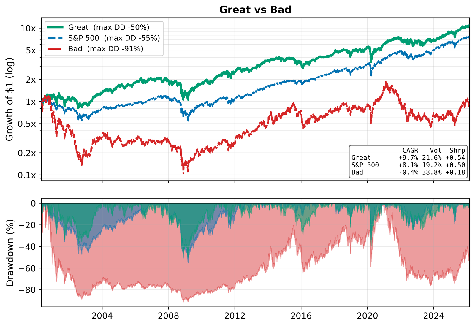
The top panel shows a dollar in each book on a log scale. The Great book climbs steadily above the S&P 500. The Bad book rides the dot-com momentum names to their peak, collapses in the bust, and never regains its early ground. The bottom panel shows why: the Bad book spends most of the sample deep underwater, with a trough of 91.3%.

Trading costs took 0.4% a year off the Great book and 1.0% a year off the Bad book. The Bad book pays more because it trades twice as much, at about 242% turnover a year against 122% for the Great book, and its failing small-cap names carry wider spreads. Costs turned the Bad book’s gross return of 0.6% a year into a net loss of 0.4%.

What this test does not settle

One specification. I ran a single version of the quality score: return on capital, operating margin, and operating earnings over assets, equal-weighted top and bottom 30, monthly. The thresholds and the portfolio size are choices, and other reasonable choices give different numbers. Buffett’s wonderful company is broader than three profitability ratios, taking in valuation, management, and future prospects, so this is only the mechanical slice of that idea. This is one path, and it does not come with a confidence interval.

The Bad book may be untradeable. The bottom 30 are unprofitable small companies with heavy losses, wide spreads, and in some months no borrow to short. A few of these names did rebound enormously off the bottom. Catching them, though, would take the timing of one of Jack Schwager’s market wizards, and a mechanical screen does not have it. The 91.3% drawdown is real in the data, and a short seller could not reliably capture the mirror image of it. The Bad book is best read as a description of where low quality leads.

Long-only, two separate books. I show the great and the bad as two long books. A long-short quality portfolio that buys one and shorts the other is a different test, with financing costs and borrow constraints this backtest does not carry.

Costs are approximate. The half-spread plus a flat commission understate real trading in small, illiquid names, which the Bad book holds. The true drag on the Bad book is higher than the 1.0% a year charged here.

Return on capital is a proxy. I use the closest field the vendor reports for return on capital, which is not identical to a hand-built version. The ranking it produces is close to the hand-built version.

What it means

Ranking US companies on three profitability measures separated the winners from the losers over 26 years. The highest-quality book compounded at 9.7% a year and beat the S&P 500 by 1.6 points. The lowest-quality book lost money and fell 91.3% at its worst. The gap held on every risk-adjusted measure and widened on the ones that count only losses. The takeaway is that quality paid on both sides, because the best companies compounded while the worst destroyed capital.

Read next

• The Magic Formula worked. Just not lately. The same quality-and-value idea, built as a mechanical stock screen.
• Just 4% of stocks created nearly all the wealth Why owning the winners, and avoiding the worst, decides a portfolio.

Disclaimer: simplified, hypothetical backtest with approximate trading costs, for discussion purposes only. Not investment advice. Past performance does not predict future returns.

Data: US equity prices, fundamentals, and bid-ask quotes from LSEG Workspace (licensed). The S&P 500 total-return series is the benchmark. I do not reproduce the raw file here.